Last updated: 2019-04-03

workflowr checks: (Click a bullet for more information)

✔ R Markdown file: up-to-date

Great! Since the R Markdown file has been committed to the Git repository, you know the exact version of the code that produced these results.
✔ Environment: empty

Great job! The global environment was empty. Objects defined in the global environment can affect the analysis in your R Markdown file in unknown ways. For reproduciblity it’s best to always run the code in an empty environment.
✔ Seed: set.seed(20190110)

The command set.seed(20190110) was run prior to running the code in the R Markdown file. Setting a seed ensures that any results that rely on randomness, e.g. subsampling or permutations, are reproducible.
✔ Session information: recorded

Great job! Recording the operating system, R version, and package versions is critical for reproducibility.

✔ Repository version: 5870e6e

Great! You are using Git for version control. Tracking code development and connecting the code version to the results is critical for reproducibility. The version displayed above was the version of the Git repository at the time these results were generated.

Note that you need to be careful to ensure that all relevant files for the analysis have been committed to Git prior to generating the results (you can use wflow_publish or wflow_git_commit). workflowr only checks the R Markdown file, but you know if there are other scripts or data files that it depends on. Below is the status of the Git repository when the results were generated:


Ignored files:
    Ignored:    .DS_Store
    Ignored:    .Rhistory
    Ignored:    .Rproj.user/
    Ignored:    ._.DS_Store
    Ignored:    analysis/cache/
    Ignored:    build-logs/
    Ignored:    data/alevin/
    Ignored:    data/cellranger/
    Ignored:    data/processed/
    Ignored:    data/published/
    Ignored:    output/.DS_Store
    Ignored:    output/._.DS_Store
    Ignored:    output/03-clustering/selected_genes.csv.zip
    Ignored:    output/04-marker-genes/de_genes.csv.zip
    Ignored:    packrat/.DS_Store
    Ignored:    packrat/._.DS_Store
    Ignored:    packrat/lib-R/
    Ignored:    packrat/lib-ext/
    Ignored:    packrat/lib/
    Ignored:    packrat/src/

Untracked files:
    Untracked:  DGEList.Rds
    Untracked:  output/90-methods/package-versions.json
    Untracked:  scripts/build.pbs

Unstaged changes:
    Modified:   analysis/_site.yml
    Modified:   output/01-preprocessing/droplet-selection.pdf
    Modified:   output/01-preprocessing/parameters.json
    Modified:   output/01-preprocessing/selection-comparison.pdf
    Modified:   output/01B-alevin/alevin-comparison.pdf
    Modified:   output/01B-alevin/parameters.json
    Modified:   output/02-quality-control/qc-thresholds.pdf
    Modified:   output/02-quality-control/qc-validation.pdf
    Modified:   output/03-clustering/cluster-comparison.pdf
    Modified:   output/03-clustering/cluster-validation.pdf
    Modified:   output/04-marker-genes/de-results.pdf

Note that any generated files, e.g. HTML, png, CSS, etc., are not included in this status report because it is ok for generated content to have uncommitted changes.

Expand here to see past versions:

File	Version	Author	Date	Message
html	33ac14f	Luke Zappia	2019-03-20	Tidy up website
html	ae75188	Luke Zappia	2019-03-06	Revise figures after proofread
html	2693e97	Luke Zappia	2019-03-05	Add methods page
html	fefdd07	Luke Zappia	2019-02-28	Add PAGA figure
Rmd	dd11830	Luke Zappia	2019-02-12	Add PAGA text
html	dd11830	Luke Zappia	2019-02-12	Add PAGA text
html	ee99ad1	Luke Zappia	2019-02-10	Add PAGA

# scRNA-seq
library("SingleCellExperiment")

# System
library("processx")

# Plotting
library("cowplot")

# Presentation
library("knitr")

# Tidyverse
library("tidyverse")

source(here::here("R/output.R"))
source(here::here("R/plotting.R"))

clust_path <- here::here("data/processed/03-clustered.Rds")
paga_path <- here::here("scripts/paga.py")

Introduction

In this document we are going to explore the relationship between our clusters using partition-based graph abstraction (PAGA). PAGA builds a graph where each node is a cluster and the edges represent connectivity between clusters. This can give us an overview of the dataset and the relationships between cell types.

if (file.exists(clust_path)) {
    sce <- read_rds(clust_path)
} else {
    stop("Clustered dataset is missing. ",
         "Please run '03-clustering.Rmd' first.",
         call. = FALSE)
}

PAGA

PAGA is available as part of the scanpy Python package. The PAGA analysis is performed using the following Python script.

cat(readLines(paga_path), sep = "\n")

#!/usr/bin/env python3

import os
import json
import numpy
import pandas as pd
import loompy
import anndata
import scanpy as sc

# Show errors (0), warnings (1), info (2) and hints (3)
sc.settings.verbosity = 3

print('Reading clustering parameters...')
params_path = 'output/03-clustering/parameters.json'

with open(params_path) as params_file:
    params = json.load(params_file)

for param in params:
    if param['Parameter'][0] == 'n_pcs':
        n_pcs = param['Value'][0]

    if param['Parameter'][0] == 'knn':
        knn = param['Value'][0]

print('Reading Loom file...')
loom_path = 'data/processed/03-clustered-sel.loom'

col_names = ['Cell', 'Barcode', 'Dataset', 'Sample', 'Cluster']
obs = dict()

with loompy.connect(loom_path) as loom_con:
    X = loom_con.layers[''][()].T

    for col in col_names:
        obs[col] = loom_con.col_attrs[col]

print('Converting to AnnData...')
adata = anndata.AnnData(X=X, obs=obs)

print('Calculating PCs...')
sc.tl.pca(adata, svd_solver='arpack')

print('Calculating neighbour graph...')
sc.pp.neighbors(adata, n_neighbors=30, n_pcs=15)

print('Perfoming PAGA...')
sc.tl.paga(adata, groups='Cluster')

print('Calculating cluster graph layout...')
sc.pl.paga(adata, plot=False)

print('Calculating cell graph layout...')
sc.tl.draw_graph(adata, init_pos='paga')

out_dir = 'output/05-paga'
if not os.path.exists(out_dir):
    os.makedirs(out_dir)

def con2edges(con, names=None, sparse=True):
    print('Converting connectivity matrix to edges...')
    n = con.shape[0]
    edges = pd.DataFrame(columns=['From', 'To', 'Connectivity'])

    for i in range(n):
        for j in range(i + 1, n):
            if names is not None:
                fr = names[i]
                to = names[j]
            else:
                fr = str(i)
                to = str(j)

            connectivity = con[i, j]
            if sparse and connectivity == 0:
                continue

            entry = {'From' : fr, 'To' : to,
                     'Connectivity' : con[i, j]}
            edges = edges.append(entry, ignore_index=True)

    return edges

print('Outputting cluster edges...')
clust_con = adata.uns['paga']['connectivities'].toarray()
clust_edges = con2edges(clust_con)
clust_edges.to_csv(os.path.join(out_dir, 'cluster_edges.csv'),
                   index=False)

print('Outputting cluster tree edges...')
clust_tree_con = adata.uns['paga']['connectivities_tree'].toarray()
clust_tree_edges = con2edges(clust_tree_con)
clust_tree_edges.to_csv(os.path.join(out_dir, 'cluster_tree_edges.csv'),
                        index=False)

print('Outputting cluster embedding...')
clust_embedding = pd.DataFrame(adata.uns['paga']['pos'], columns=['X', 'Y'])
clust_embedding['Cluster'] = range(clust_embedding.shape[0])
clust_embedding = clust_embedding[['Cluster', 'X', 'Y']]

clust_embedding.to_csv(os.path.join(out_dir, 'cluster_embedding.csv'),
                       index=False)

print('Outputting cell edges...')
cells = adata.obs['Cell']
cell_con = adata.uns['neighbors']['connectivities']
cell_edges = pd.DataFrame(columns=['From', 'To', 'Connectivity'])
n_rows = len(cell_con.indptr)

for i in range(len(cell_con.indptr) - 1):
    row_ind = cell_con.indices[cell_con.indptr[i]:cell_con.indptr[i + 1]]
    print(f'\r\tRow {i} of {n_rows}', end='')
    for k, j in enumerate(row_ind):
        if j > i:
            con = cell_con.data[cell_con.indptr[i] + k]
            fr = cells[i]
            to = cells[j]
            entry = {'From' : fr, 'To' : to, 'Connectivity' : con}
            cell_edges = cell_edges.append(entry, ignore_index=True)
print('\n')

cell_edges.to_csv(os.path.join(out_dir, 'cell_edges.csv'),
                  index=False)

print('Outputting cell embedding...')
x = adata.obsm['X_draw_graph_fa'][:, 0]
y = adata.obsm['X_draw_graph_fa'][:, 1]
cell_embedding = pd.DataFrame({'Cell' : cells, 'X' : x, 'Y' : y})
cell_embedding.to_csv(os.path.join(out_dir, 'cell_embedding.csv'),
                      index=False)

print('Done!')

paga_out <- run(here::here("scripts/run_paga.sh"))

We then load the PAGA results and visualise them here.

clust_embedding <- read_csv(
    here::here("output/05-paga/cluster_embedding.csv"),
    col_types = cols(
        .default = col_double()
    )
) %>%
    mutate(Size = as.numeric(table(colData(sce)$Cluster))) %>%
    mutate(Cluster = factor(Cluster, levels = levels(colData(sce)$Cluster)))

clust_edges <- read_csv(
    here::here("output/05-paga/cluster_edges.csv"),
    col_types = cols(
        .default = col_double()
    )
) %>%
    mutate(To = factor(To, levels = levels(colData(sce)$Cluster)),
           From = factor(From, levels = levels(colData(sce)$Cluster))) %>%
    left_join(clust_embedding, by = c("From" = "Cluster")) %>%
    rename(FromX = X, FromY = Y) %>%
    select(-Size) %>%
    left_join(clust_embedding, by = c("To" = "Cluster")) %>%
    rename(ToX = X, ToY = Y) %>%
    select(-Size)

cell_embedding <- read_csv(
    here::here("output/05-paga/cell_embedding.csv"),
    col_types = cols(
        .default = col_double(),
        Cell = col_character()
    )
) %>%
    mutate(Cluster = colData(sce)$Cluster)

cell_edges <- read_csv(
    here::here("output/05-paga/cell_edges.csv"),
    col_types = cols(
        .default = col_double(),
        From = col_character(),
        To = col_character()
    )
) %>%
    left_join(cell_embedding, by = c("From" = "Cell")) %>%
    rename(FromX = X, FromY = Y) %>%
    select(-Cluster) %>%
    left_join(cell_embedding, by = c("To" = "Cell")) %>%
    rename(ToX = X, ToY = Y) %>%
    select(-Cluster)

Cluster graph

The PAGA graph shows the relationship between clusters. Here we have use a force directed graph layout in order to visualise it. PAGA calculates the connectivity between each pair of clusters but we need to apply some threshold to that to select the meaningful edges.

Thresholds

src_list <- lapply(seq(0, 0.9, 0.1), function(thresh) {
    src <- c(
        "### Con {{thresh}} {.unnumbered}",
        "```{r clust-paga-{{thresh}}}",
        "plotPAGAClustGraph(clust_embedding, clust_edges, thresh = {{thresh}})",  
        "```",
        ""
    )
    knit_expand(text = src)
})

out <- knit_child(text = unlist(src_list), options = list(cache = FALSE))

Con 0

plotPAGAClustGraph(clust_embedding, clust_edges, thresh = 0)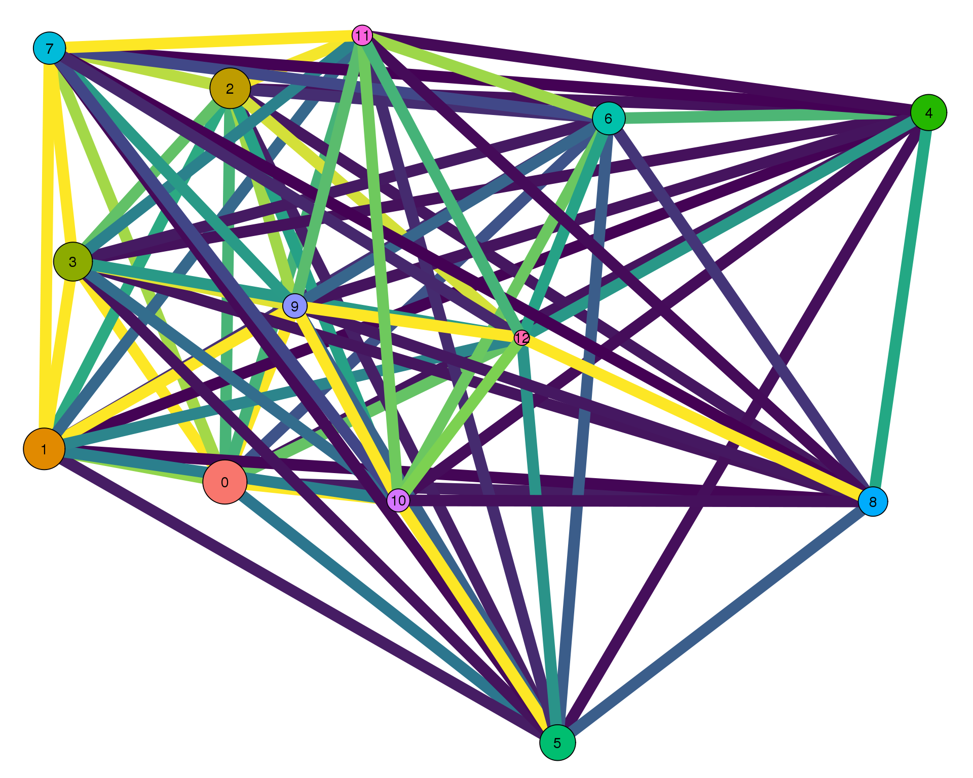

Expand here to see past versions of clust-paga-0-1.png:

Version	Author	Date
fefdd07	Luke Zappia	2019-02-28

Con 0.1

plotPAGAClustGraph(clust_embedding, clust_edges, thresh = 0.1)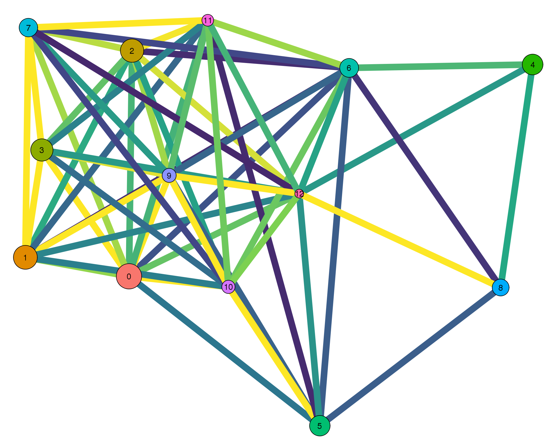

Expand here to see past versions of clust-paga-0.1-1.png:

Version	Author	Date
fefdd07	Luke Zappia	2019-02-28

Con 0.2

plotPAGAClustGraph(clust_embedding, clust_edges, thresh = 0.2)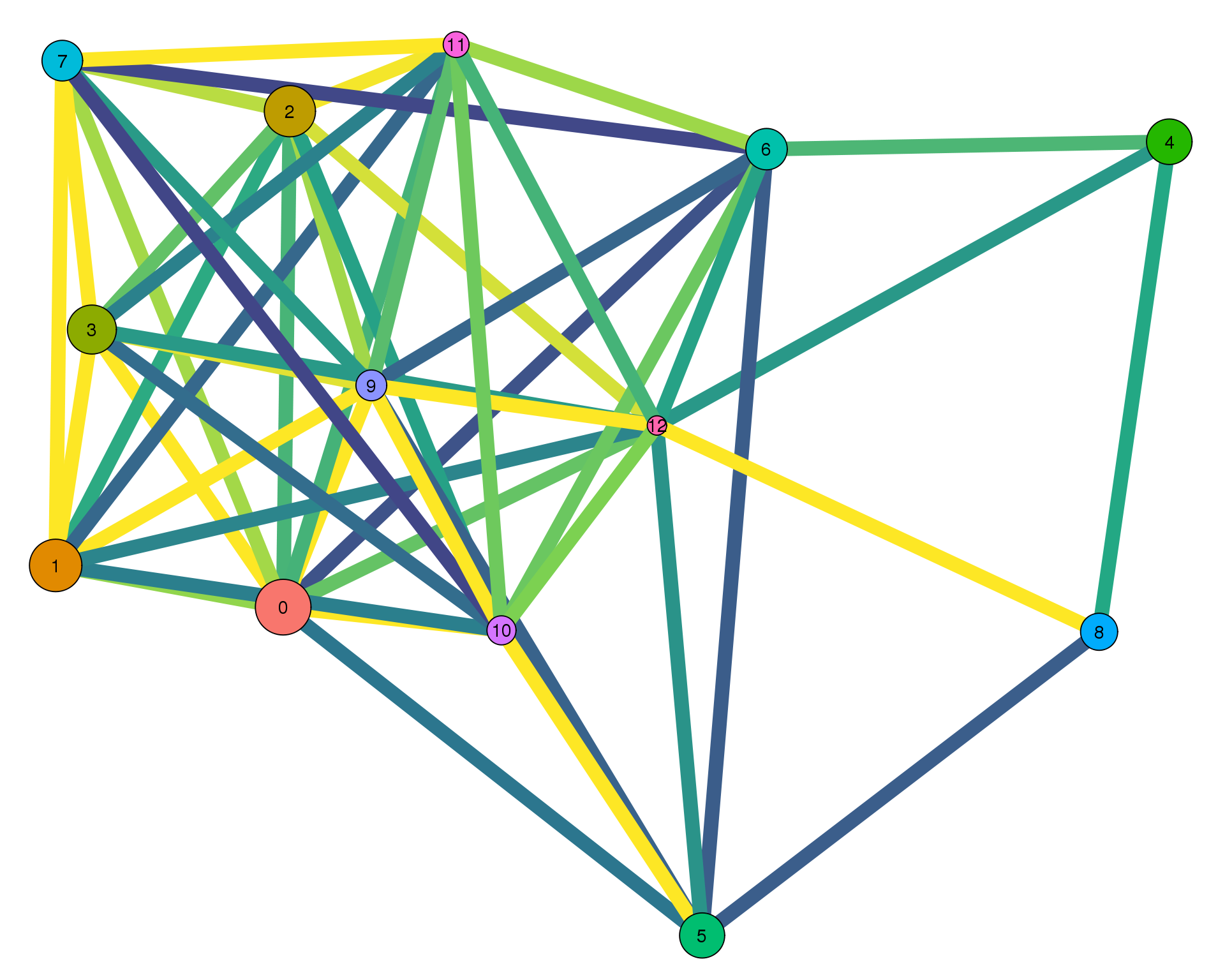

Expand here to see past versions of clust-paga-0.2-1.png:

Version	Author	Date
fefdd07	Luke Zappia	2019-02-28

Con 0.3

plotPAGAClustGraph(clust_embedding, clust_edges, thresh = 0.3)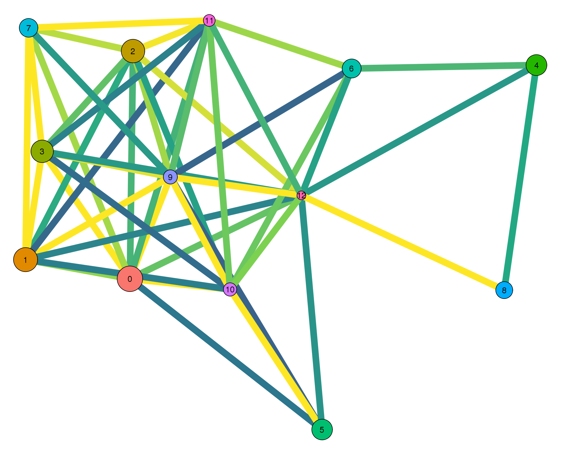

Expand here to see past versions of clust-paga-0.3-1.png:

Version	Author	Date
fefdd07	Luke Zappia	2019-02-28

Con 0.4

plotPAGAClustGraph(clust_embedding, clust_edges, thresh = 0.4)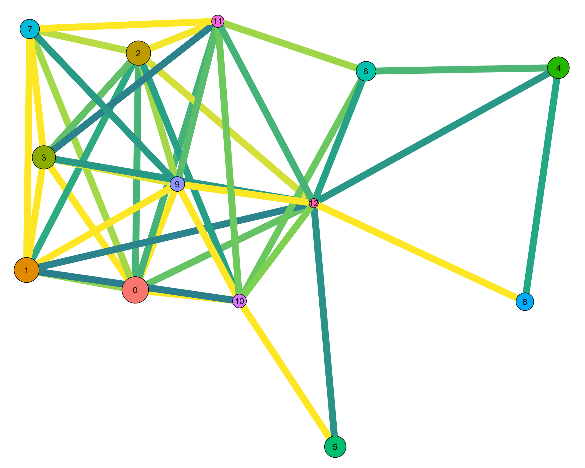

Expand here to see past versions of clust-paga-0.4-1.png:

Version	Author	Date
fefdd07	Luke Zappia	2019-02-28

Con 0.5

plotPAGAClustGraph(clust_embedding, clust_edges, thresh = 0.5)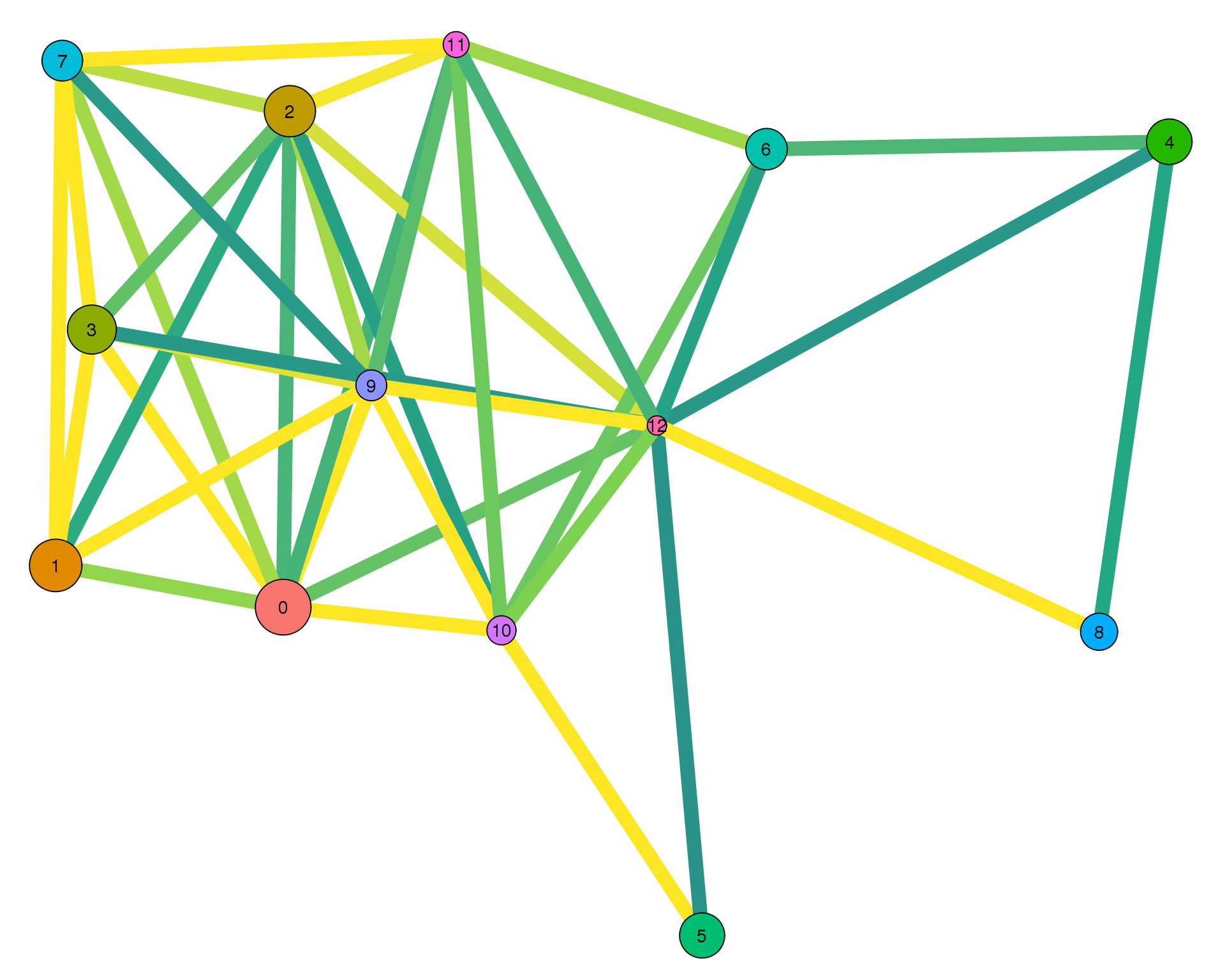

Expand here to see past versions of clust-paga-0.5-1.png:

Version	Author	Date
fefdd07	Luke Zappia	2019-02-28

Con 0.6

plotPAGAClustGraph(clust_embedding, clust_edges, thresh = 0.6)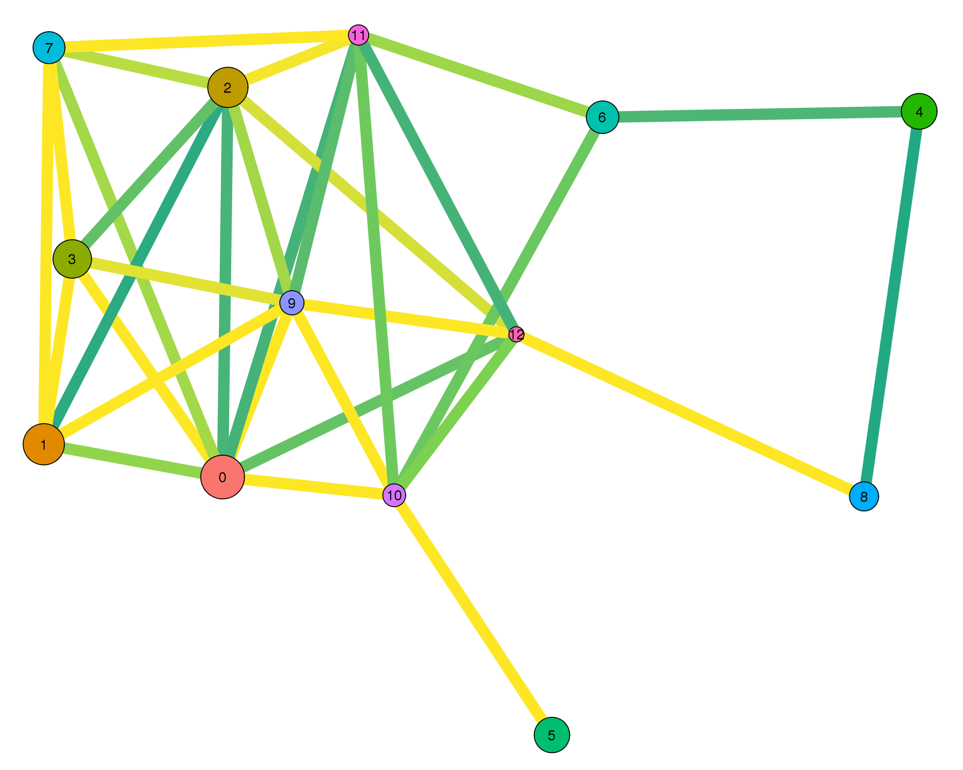

Expand here to see past versions of clust-paga-0.6-1.png:

Version	Author	Date
fefdd07	Luke Zappia	2019-02-28

Con 0.7

plotPAGAClustGraph(clust_embedding, clust_edges, thresh = 0.7)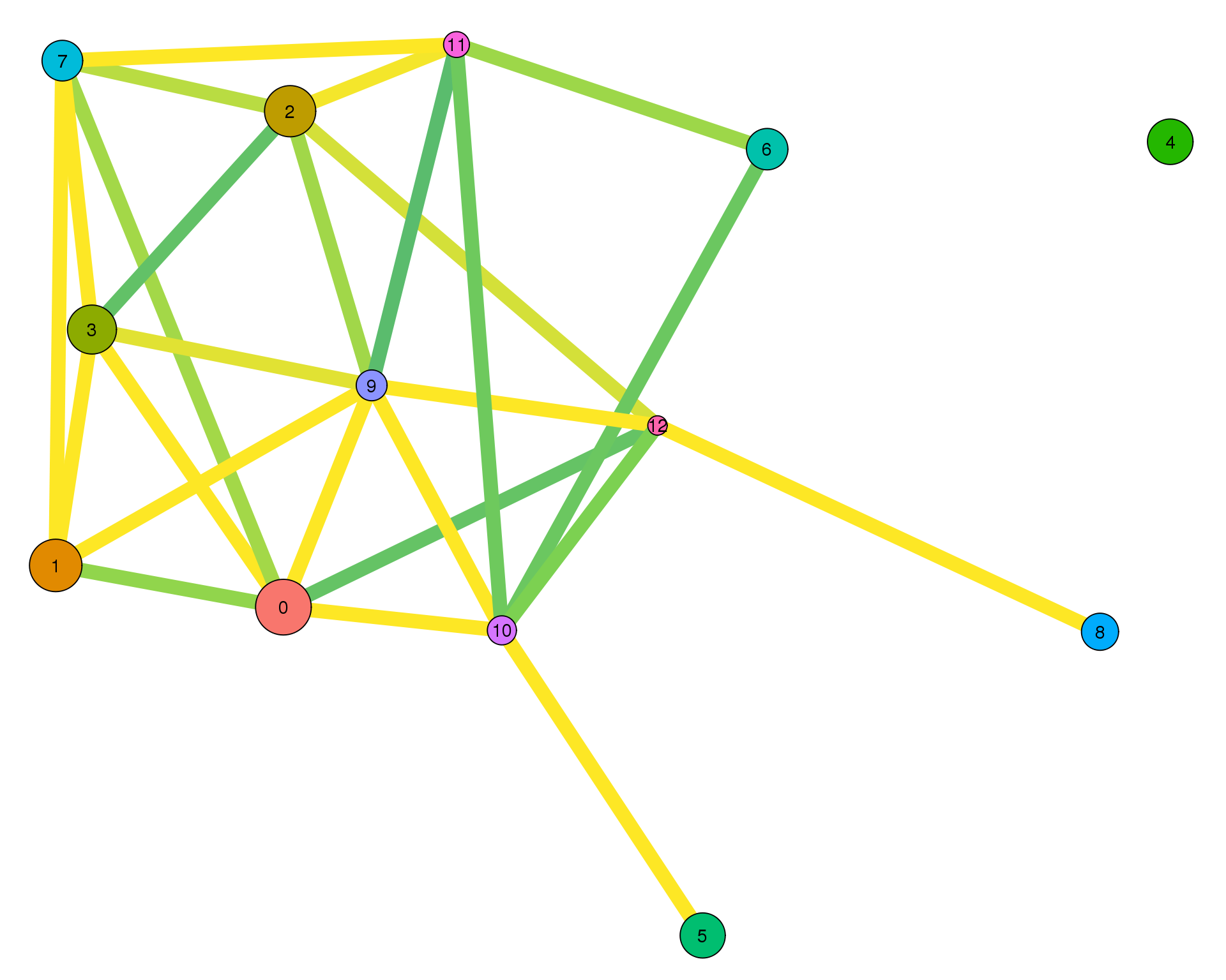

Expand here to see past versions of clust-paga-0.7-1.png:

Version	Author	Date
fefdd07	Luke Zappia	2019-02-28

Con 0.8

plotPAGAClustGraph(clust_embedding, clust_edges, thresh = 0.8)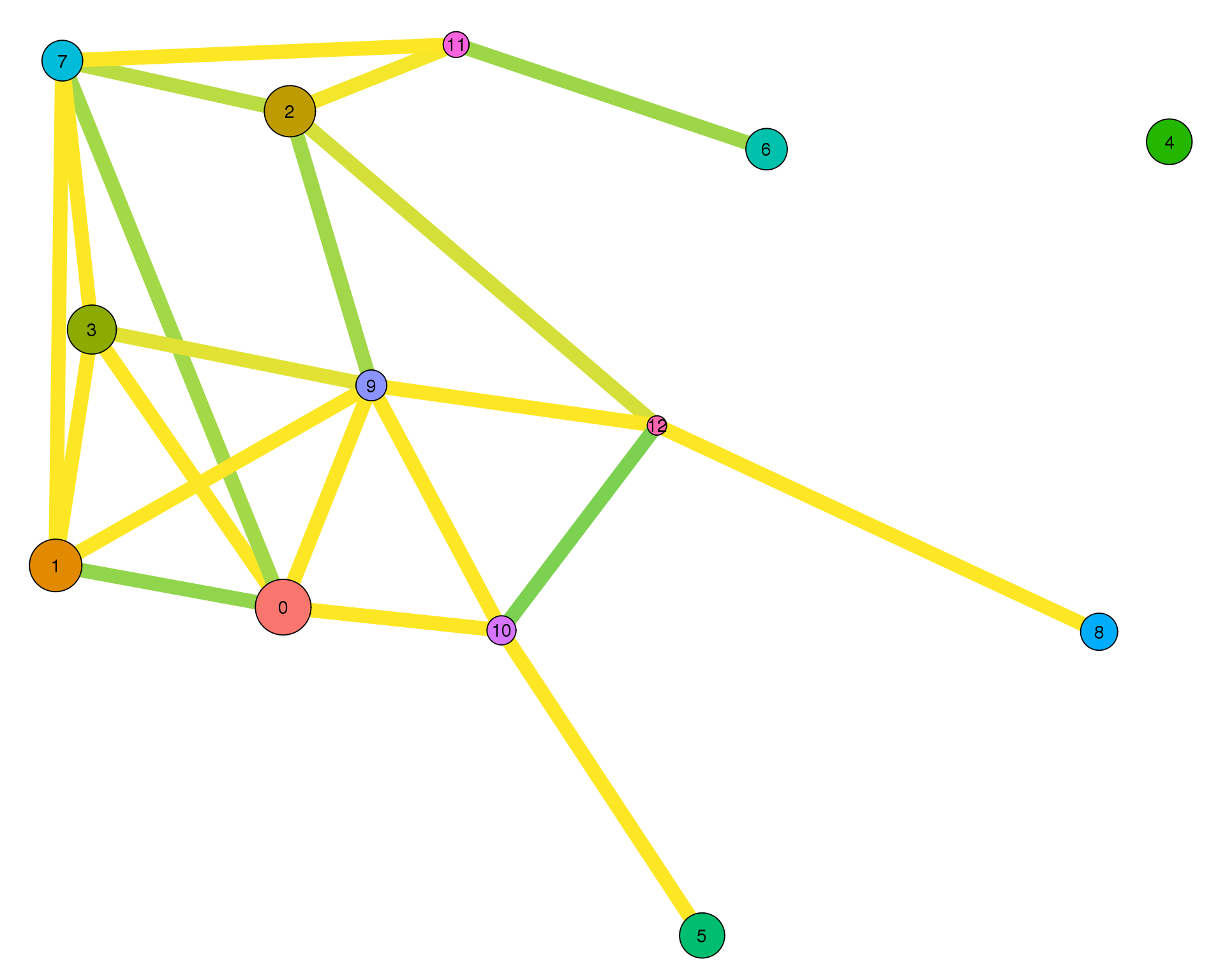

Expand here to see past versions of clust-paga-0.8-1.png:

Version	Author	Date
fefdd07	Luke Zappia	2019-02-28

Con 0.9

plotPAGAClustGraph(clust_embedding, clust_edges, thresh = 0.9)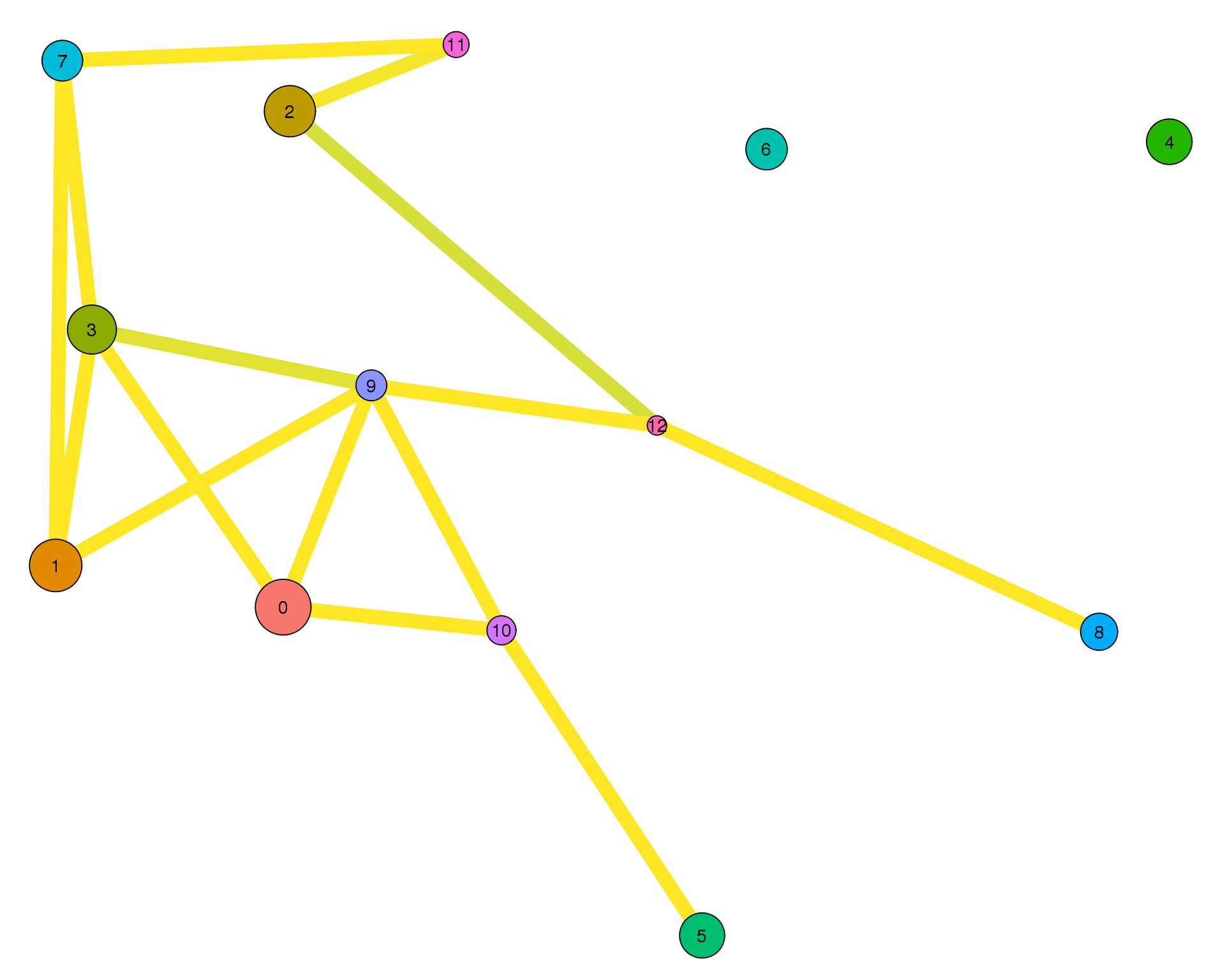

Expand here to see past versions of clust-paga-0.9-1.png:

Version	Author	Date
fefdd07	Luke Zappia	2019-02-28

Edges by threshold

Number of selected edges for different threshold connectivities.

plot_data <- tibble(
    Threshold = seq(0, 1, 0.01)
) %>%
    mutate(Edges = map_int(Threshold, function(thresh) {
        sum(clust_edges$Connectivity > thresh)
    }))

con_thresh <- 0.7

ggplot(plot_data, aes(x = Threshold, y = Edges)) +
    geom_point() +
    geom_line() +
    geom_vline(xintercept = con_thresh, colour = "red") +
    xlab("Connectivity threshold") +
    ylab("Number of edges") +
    theme_minimal()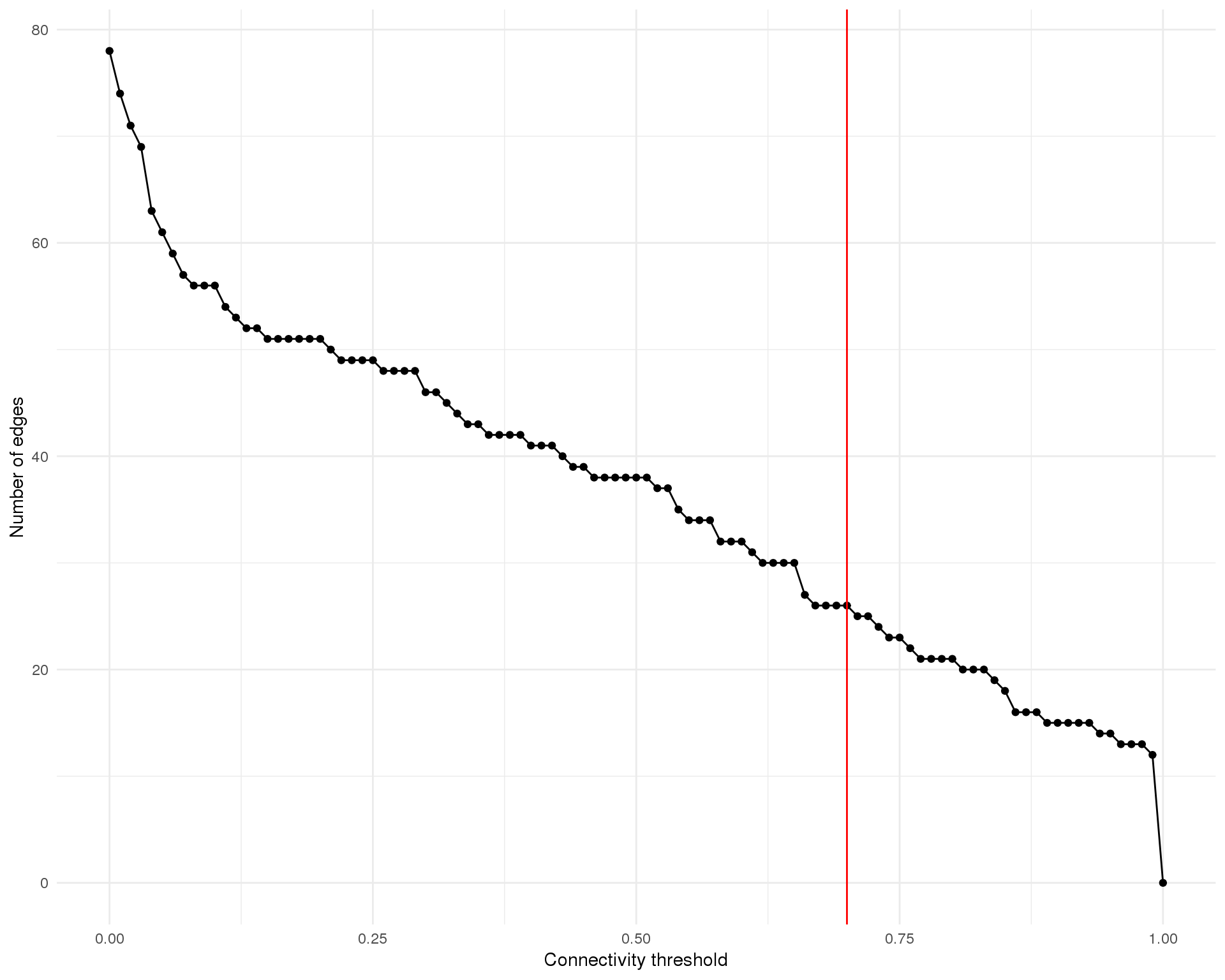

Expand here to see past versions of thresh-edges-1.png:

Version	Author	Date
fefdd07	Luke Zappia	2019-02-28

Here we have selected a connectivity threshold of 0.7.

Cell graph

The cluster graph can be used as a starting point to layout individual cells, allowing us to see things at a higher resolution.

plotPAGACellGraph(cell_embedding, cell_edges, thresh = 0.1)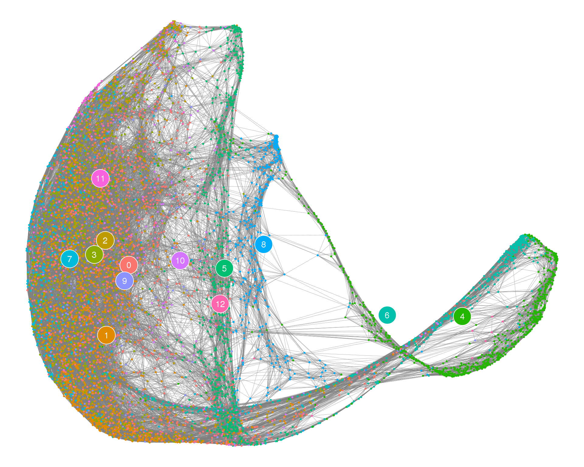

Expand here to see past versions of cell-paga-1.png:

Version	Author	Date
fefdd07	Luke Zappia	2019-02-28

Compare

Looking the two views together let’s us see both global and specific details.

plotPAGACompare(clust_embedding, clust_edges, clust_thresh = con_thresh,
                cell_embedding, cell_edges, cell_thresh = 0.1)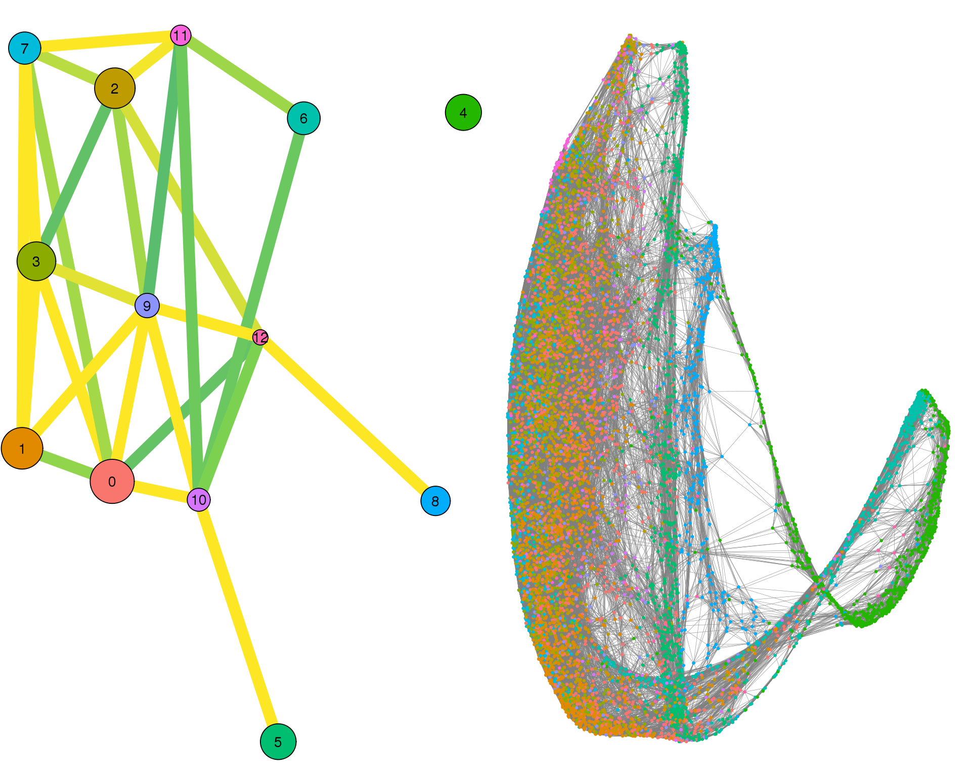

Expand here to see past versions of compare-paga-1.png:

Version	Author	Date
fefdd07	Luke Zappia	2019-02-28

Genes

known_genes <- c(
    # Stroma
    "TAGLN", "ACTA2", "MAB21L2", "DLK1", "GATA3", "COL2A1", "COL9A3",
    # Podocyte
    "PODXL", "NPHS2", "TCF21",
    # Cell cycle
    "HIST1H4C", "PCLAF", "CENPF", "HMGB2",
    # Endothelium
    "CLDN5", "PECAM1", "KDR", "CALM1",
    # Neural
    "TTYH1", "SOX2", "HES6", "STMN2",
    # Epithelium
    "PAX2", "PAX8", "KRT19",
    # Muscle
    "MYOG", "MYOD1"
)

for (gene in known_genes) {
    cell_embedding[[gene]] <- logcounts(sce)[gene, ]
}

clust_genes <- cell_embedding %>%
    select(-Cell, -X, -Y) %>%
    group_by(Cluster) %>%
    summarise_all(mean)

clust_embedding <- left_join(clust_embedding, clust_genes, by = "Cluster")

src_list <- lapply(known_genes, function(gene) {
    src <- c(
        "### {{gene}} {.unnumbered}",
        "```{r compare-{{gene}}}",
        "plotPAGACompare(clust_embedding, clust_edges,",
        "clust_thresh = con_thresh, cell_embedding, cell_edges,
        cell_thresh = 0.1, colour = '{{gene}}')",  
        "```",
        ""
    )
    knit_expand(text = src)
})

out <- knit_child(text = unlist(src_list), options = list(cache = FALSE))

TAGLN

plotPAGACompare(clust_embedding, clust_edges,
clust_thresh = con_thresh, cell_embedding, cell_edges,
        cell_thresh = 0.1, colour = 'TAGLN')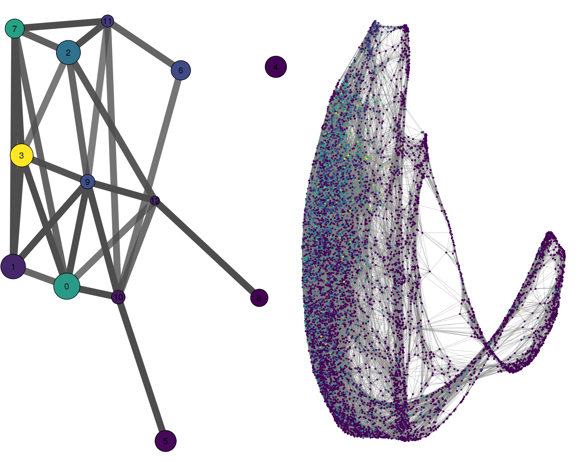

Expand here to see past versions of compare-TAGLN-1.png:

Version	Author	Date
fefdd07	Luke Zappia	2019-02-28

ACTA2

plotPAGACompare(clust_embedding, clust_edges,
clust_thresh = con_thresh, cell_embedding, cell_edges,
        cell_thresh = 0.1, colour = 'ACTA2')

Expand here to see past versions of compare-ACTA2-1.png:

Version	Author	Date
fefdd07	Luke Zappia	2019-02-28

MAB21L2

plotPAGACompare(clust_embedding, clust_edges,
clust_thresh = con_thresh, cell_embedding, cell_edges,
        cell_thresh = 0.1, colour = 'MAB21L2')

Expand here to see past versions of compare-MAB21L2-1.png:

Version	Author	Date
fefdd07	Luke Zappia	2019-02-28

DLK1

plotPAGACompare(clust_embedding, clust_edges,
clust_thresh = con_thresh, cell_embedding, cell_edges,
        cell_thresh = 0.1, colour = 'DLK1')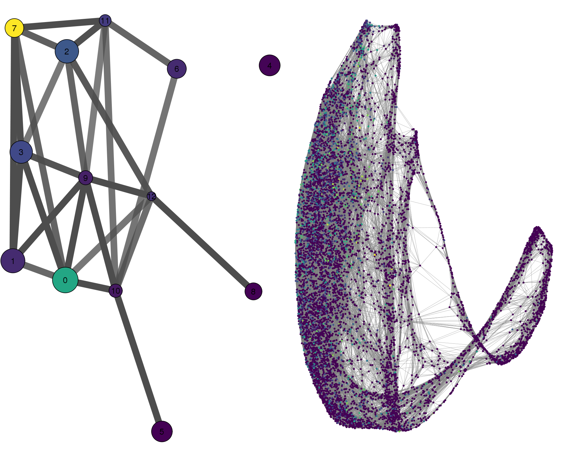

Expand here to see past versions of compare-DLK1-1.png:

Version	Author	Date
fefdd07	Luke Zappia	2019-02-28

GATA3

plotPAGACompare(clust_embedding, clust_edges,
clust_thresh = con_thresh, cell_embedding, cell_edges,
        cell_thresh = 0.1, colour = 'GATA3')

Expand here to see past versions of compare-GATA3-1.png:

Version	Author	Date
fefdd07	Luke Zappia	2019-02-28

COL2A1

plotPAGACompare(clust_embedding, clust_edges,
clust_thresh = con_thresh, cell_embedding, cell_edges,
        cell_thresh = 0.1, colour = 'COL2A1')

Expand here to see past versions of compare-COL2A1-1.png:

Version	Author	Date
fefdd07	Luke Zappia	2019-02-28

COL9A3

plotPAGACompare(clust_embedding, clust_edges,
clust_thresh = con_thresh, cell_embedding, cell_edges,
        cell_thresh = 0.1, colour = 'COL9A3')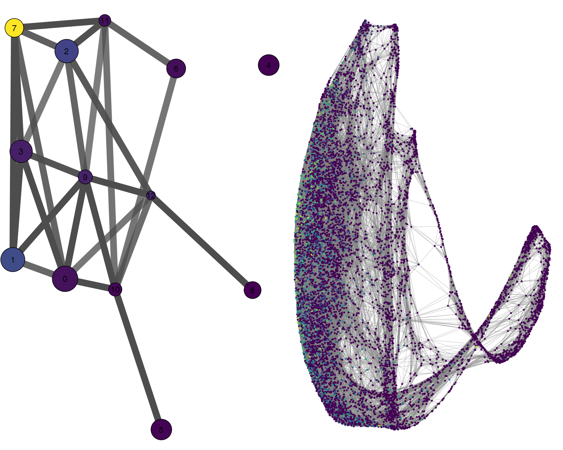

Expand here to see past versions of compare-COL9A3-1.png:

Version	Author	Date
fefdd07	Luke Zappia	2019-02-28

PODXL

plotPAGACompare(clust_embedding, clust_edges,
clust_thresh = con_thresh, cell_embedding, cell_edges,
        cell_thresh = 0.1, colour = 'PODXL')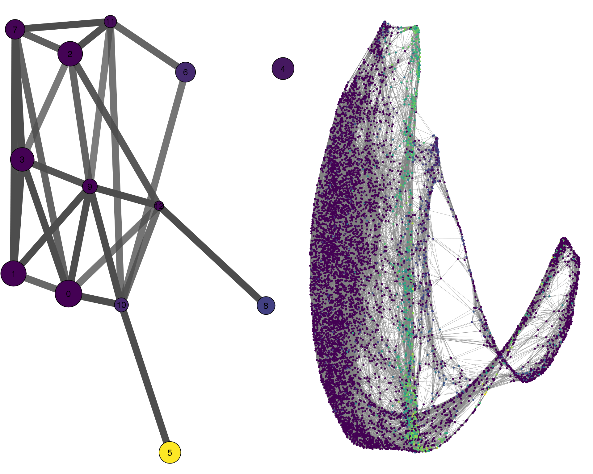

Expand here to see past versions of compare-PODXL-1.png:

Version	Author	Date
fefdd07	Luke Zappia	2019-02-28

NPHS2

plotPAGACompare(clust_embedding, clust_edges,
clust_thresh = con_thresh, cell_embedding, cell_edges,
        cell_thresh = 0.1, colour = 'NPHS2')

Expand here to see past versions of compare-NPHS2-1.png:

Version	Author	Date
fefdd07	Luke Zappia	2019-02-28

TCF21

plotPAGACompare(clust_embedding, clust_edges,
clust_thresh = con_thresh, cell_embedding, cell_edges,
        cell_thresh = 0.1, colour = 'TCF21')

Expand here to see past versions of compare-TCF21-1.png:

Version	Author	Date
fefdd07	Luke Zappia	2019-02-28

HIST1H4C

plotPAGACompare(clust_embedding, clust_edges,
clust_thresh = con_thresh, cell_embedding, cell_edges,
        cell_thresh = 0.1, colour = 'HIST1H4C')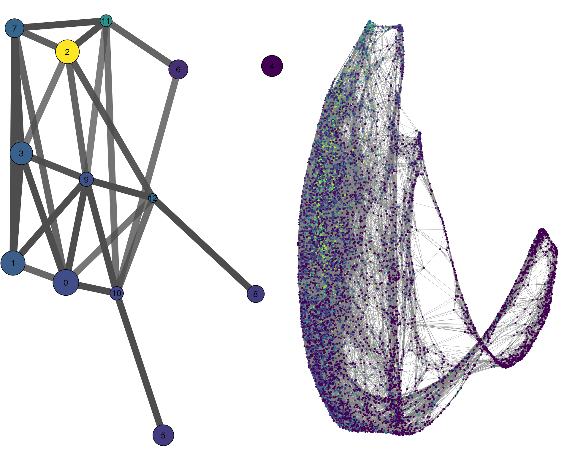

Expand here to see past versions of compare-HIST1H4C-1.png:

Version	Author	Date
fefdd07	Luke Zappia	2019-02-28

PCLAF

plotPAGACompare(clust_embedding, clust_edges,
clust_thresh = con_thresh, cell_embedding, cell_edges,
        cell_thresh = 0.1, colour = 'PCLAF')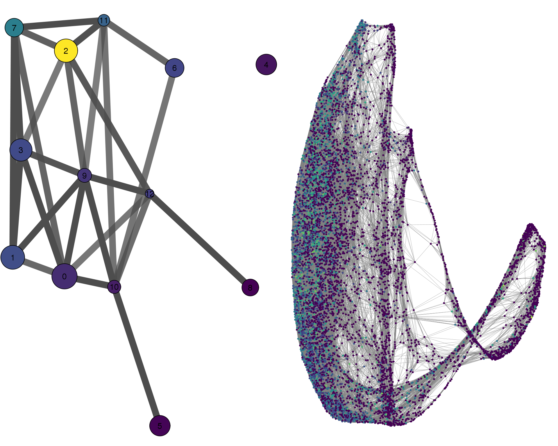

Expand here to see past versions of compare-PCLAF-1.png:

Version	Author	Date
fefdd07	Luke Zappia	2019-02-28

CENPF

plotPAGACompare(clust_embedding, clust_edges,
clust_thresh = con_thresh, cell_embedding, cell_edges,
        cell_thresh = 0.1, colour = 'CENPF')

Expand here to see past versions of compare-CENPF-1.png:

Version	Author	Date
fefdd07	Luke Zappia	2019-02-28

HMGB2

plotPAGACompare(clust_embedding, clust_edges,
clust_thresh = con_thresh, cell_embedding, cell_edges,
        cell_thresh = 0.1, colour = 'HMGB2')

Expand here to see past versions of compare-HMGB2-1.png:

Version	Author	Date
fefdd07	Luke Zappia	2019-02-28

CLDN5

plotPAGACompare(clust_embedding, clust_edges,
clust_thresh = con_thresh, cell_embedding, cell_edges,
        cell_thresh = 0.1, colour = 'CLDN5')

Expand here to see past versions of compare-CLDN5-1.png:

Version	Author	Date
fefdd07	Luke Zappia	2019-02-28

PECAM1

plotPAGACompare(clust_embedding, clust_edges,
clust_thresh = con_thresh, cell_embedding, cell_edges,
        cell_thresh = 0.1, colour = 'PECAM1')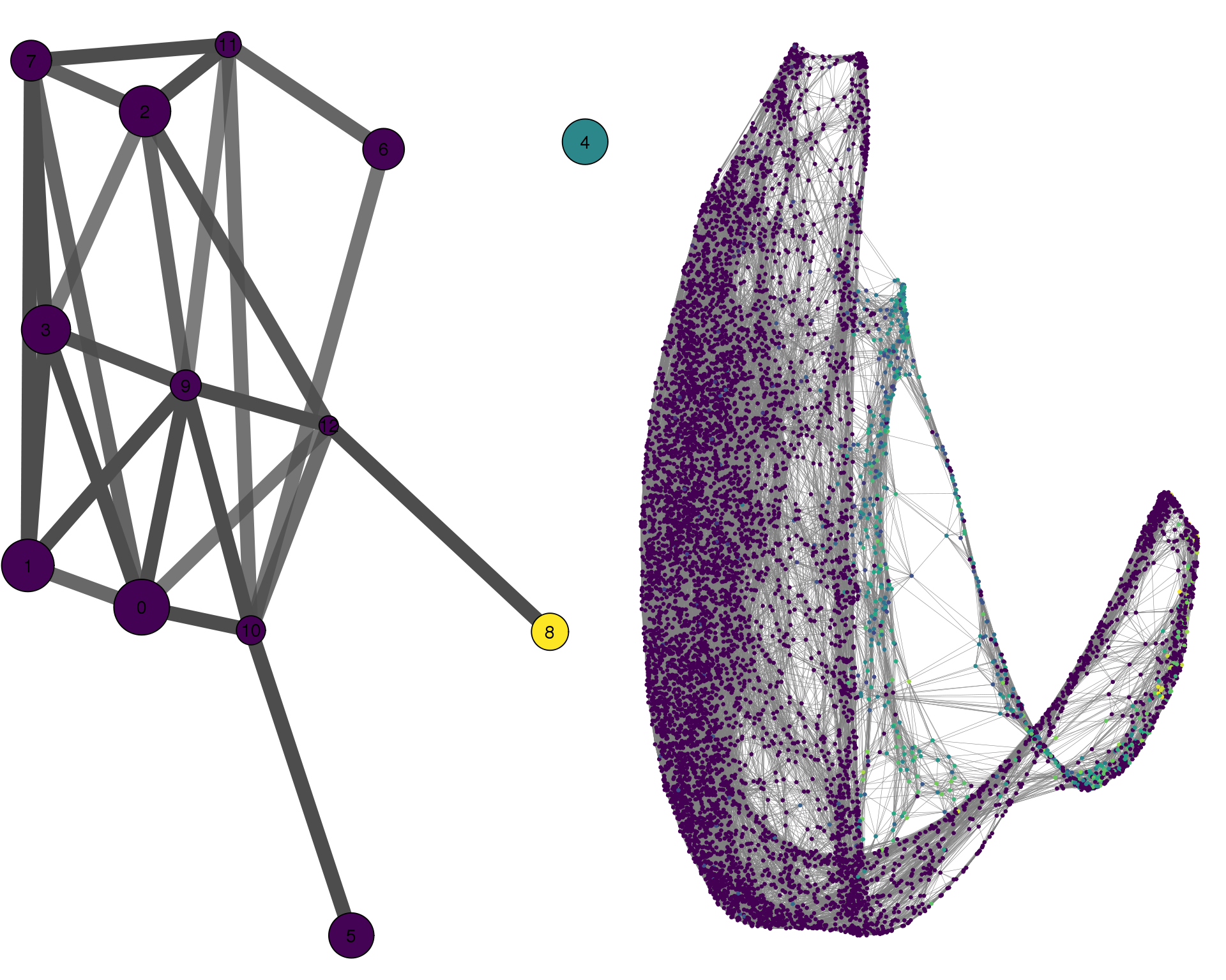

Expand here to see past versions of compare-PECAM1-1.png:

Version	Author	Date
fefdd07	Luke Zappia	2019-02-28

KDR

plotPAGACompare(clust_embedding, clust_edges,
clust_thresh = con_thresh, cell_embedding, cell_edges,
        cell_thresh = 0.1, colour = 'KDR')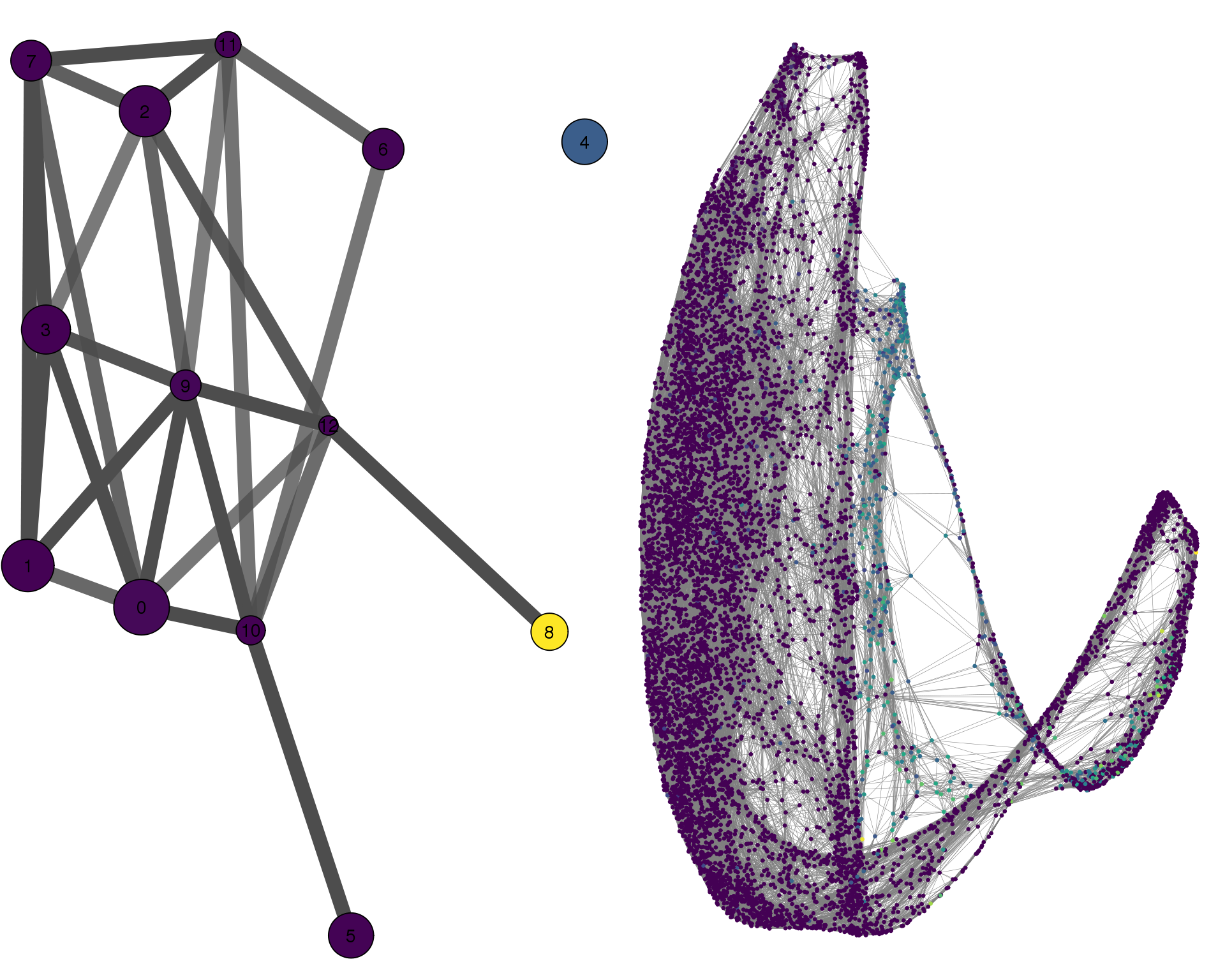

Expand here to see past versions of compare-KDR-1.png:

Version	Author	Date
fefdd07	Luke Zappia	2019-02-28

CALM1

plotPAGACompare(clust_embedding, clust_edges,
clust_thresh = con_thresh, cell_embedding, cell_edges,
        cell_thresh = 0.1, colour = 'CALM1')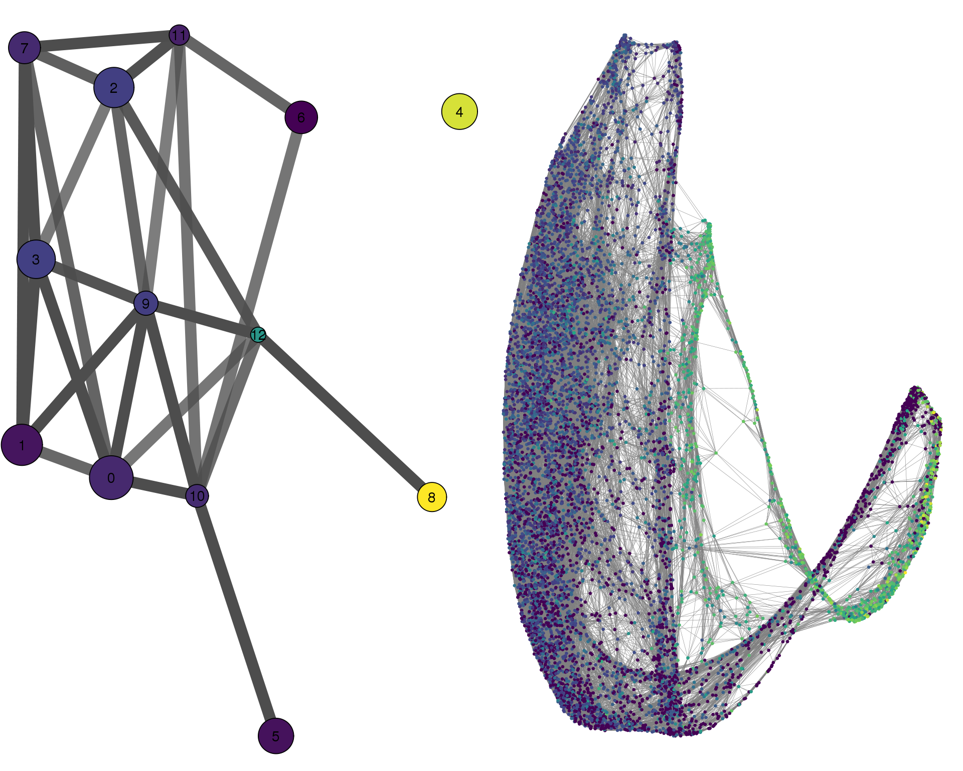

Expand here to see past versions of compare-CALM1-1.png:

Version	Author	Date
fefdd07	Luke Zappia	2019-02-28

TTYH1

plotPAGACompare(clust_embedding, clust_edges,
clust_thresh = con_thresh, cell_embedding, cell_edges,
        cell_thresh = 0.1, colour = 'TTYH1')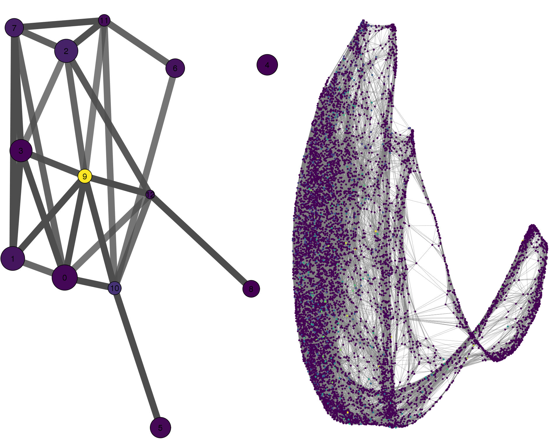

Expand here to see past versions of compare-TTYH1-1.png:

Version	Author	Date
fefdd07	Luke Zappia	2019-02-28

SOX2

plotPAGACompare(clust_embedding, clust_edges,
clust_thresh = con_thresh, cell_embedding, cell_edges,
        cell_thresh = 0.1, colour = 'SOX2')

Expand here to see past versions of compare-SOX2-1.png:

Version	Author	Date
fefdd07	Luke Zappia	2019-02-28

HES6

plotPAGACompare(clust_embedding, clust_edges,
clust_thresh = con_thresh, cell_embedding, cell_edges,
        cell_thresh = 0.1, colour = 'HES6')

Expand here to see past versions of compare-HES6-1.png:

Version	Author	Date
fefdd07	Luke Zappia	2019-02-28

STMN2

plotPAGACompare(clust_embedding, clust_edges,
clust_thresh = con_thresh, cell_embedding, cell_edges,
        cell_thresh = 0.1, colour = 'STMN2')

Expand here to see past versions of compare-STMN2-1.png:

Version	Author	Date
fefdd07	Luke Zappia	2019-02-28

PAX2

plotPAGACompare(clust_embedding, clust_edges,
clust_thresh = con_thresh, cell_embedding, cell_edges,
        cell_thresh = 0.1, colour = 'PAX2')

Expand here to see past versions of compare-PAX2-1.png:

Version	Author	Date
fefdd07	Luke Zappia	2019-02-28

PAX8

plotPAGACompare(clust_embedding, clust_edges,
clust_thresh = con_thresh, cell_embedding, cell_edges,
        cell_thresh = 0.1, colour = 'PAX8')

Expand here to see past versions of compare-PAX8-1.png:

Version	Author	Date
fefdd07	Luke Zappia	2019-02-28

KRT19

plotPAGACompare(clust_embedding, clust_edges,
clust_thresh = con_thresh, cell_embedding, cell_edges,
        cell_thresh = 0.1, colour = 'KRT19')

Expand here to see past versions of compare-KRT19-1.png:

Version	Author	Date
fefdd07	Luke Zappia	2019-02-28

MYOG

plotPAGACompare(clust_embedding, clust_edges,
clust_thresh = con_thresh, cell_embedding, cell_edges,
        cell_thresh = 0.1, colour = 'MYOG')

Expand here to see past versions of compare-MYOG-1.png:

Version	Author	Date
fefdd07	Luke Zappia	2019-02-28

MYOD1

plotPAGACompare(clust_embedding, clust_edges,
clust_thresh = con_thresh, cell_embedding, cell_edges,
        cell_thresh = 0.1, colour = 'MYOD1')

Expand here to see past versions of compare-MYOD1-1.png:

Version	Author	Date
fefdd07	Luke Zappia	2019-02-28

Figures

clust_plot <- ggplot(clust_embedding, aes(x = X, y = Y)) +
    geom_segment(data = clust_edges,
                 aes(x = FromX, y = FromY, xend = ToX, yend = ToY,
                     colour = Connectivity, alpha = Connectivity), size = 4) +
    scale_colour_viridis_c(limits = c(0, 1)) +
    scale_alpha_continuous(limits = c(0, 1), range = c(0, 1), guide = FALSE) +
    geom_point(aes(fill = Cluster, size = Size), shape = 21) +
    geom_text(aes(label = Cluster)) +
    scale_size(range = c(6, 20), guide = FALSE) +
    scale_fill_discrete(guide = FALSE) +
    guides(colour = guide_colourbar(barwidth = 20)) +
    ggtitle("PAGA cluster graph") +
    theme_void() +
    theme(plot.title = element_text(size = rel(1.2), hjust = 0.1, 
                                    vjust = 1, margin = margin(5)),
          legend.position = "bottom")

cell_plot <- ggplot(cell_embedding, aes(x = X, y = Y)) +
    geom_segment(data = cell_edges,
                 aes(x = FromX, y = FromY, xend = ToX, yend = ToY,
                     size = Connectivity, alpha = Connectivity)) +
    geom_point(aes(colour = Cluster), size = 1) +
    scale_alpha_continuous(limits = c(0, 1), range = c(0, 0.5), guide = FALSE) +
    scale_colour_discrete(guide = guide_legend(
        nrow = 1, override.aes = list(size = 4)
    )) +
    scale_size(range = c(0.1, 0.5), guide = FALSE) +
    ggtitle("Cell shared nearest neighbour graph") +
    theme_void() +
    theme(plot.title = element_text(size = rel(1.2), hjust = 0.1, 
                                    vjust = 1, margin = margin(5)),
          legend.position = "bottom")

fig <- plot_grid(clust_plot, cell_plot, nrow = 2, labels = "AUTO")

ggsave(here::here("output", DOCNAME, "paga-results.pdf"), fig,
       width = 7, height = 8, scale = 1.5)
ggsave(here::here("output", DOCNAME, "paga-results.png"), fig,
       width = 7, height = 8, scale = 1.5)

fig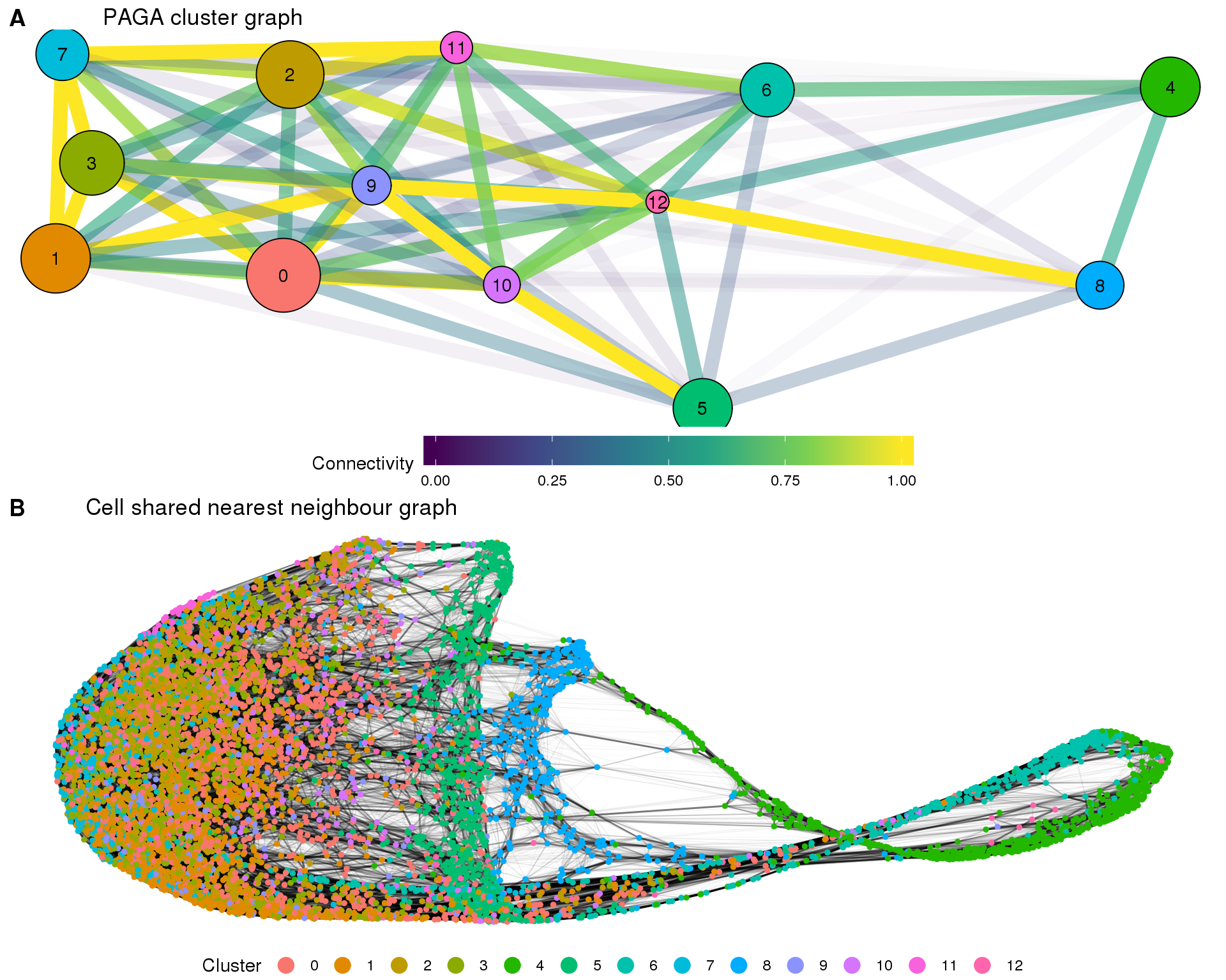

Expand here to see past versions of figure-1.png:

Version	Author	Date
2693e97	Luke Zappia	2019-03-05
fefdd07	Luke Zappia	2019-02-28

Summary

Parameters

This table describes parameters used and set in this document.

params <- list(
    list(
        Parameter = "con_thresh",
        Value = con_thresh,
        Description = "Connectivity threshold for PAGA graph"
    )
)

params <- jsonlite::toJSON(params, pretty = TRUE)
knitr::kable(jsonlite::fromJSON(params))

Parameter	Value	Description
con_thresh	0.7	Connectivity threshold for PAGA graph

Output files

This table describes the output files produced by this document. Right click and Save Link As… to download the results.

dir.create(here::here("output", DOCNAME), showWarnings = FALSE)

readr::write_lines(params, here::here("output", DOCNAME, "parameters.json"))

knitr::kable(data.frame(
    File = c(
        getDownloadLink("parameters.json", DOCNAME),
        getDownloadLink("cluster_embedding.csv", DOCNAME),
        getDownloadLink("cluster_edges.csv", DOCNAME),
        getDownloadLink("cluster_tree_edges.csv", DOCNAME),
        getDownloadLink("cell_embedding.csv", DOCNAME),
        getDownloadLink("cell_edges.csv", DOCNAME),
        getDownloadLink("paga-results.png", DOCNAME),
        getDownloadLink("paga-results.pdf", DOCNAME)
    ),
    Description = c(
        "Parameters set and used in this analysis",
        "Embedding for clusters from PAGA",
        "Edges for PAGA cluster graph",
        "Tree edges for PAGA cluster graph",
        "Embedding for cells from PAGA",
        "Edges for cell graph",
        "PAGA results figure (PNG)",
        "PAGA results figure (PDF)"
    )
))

File	Description
parameters.json	Parameters set and used in this analysis
cluster_embedding.csv	Embedding for clusters from PAGA
cluster_edges.csv	Edges for PAGA cluster graph
cluster_tree_edges.csv	Tree edges for PAGA cluster graph
cell_embedding.csv	Embedding for cells from PAGA
cell_edges.csv	Edges for cell graph
paga-results.png	PAGA results figure (PNG)
paga-results.pdf	PAGA results figure (PDF)

Session information

devtools::session_info()

─ Session info ──────────────────────────────────────────────────────────
 setting  value                       
 version  R version 3.5.0 (2018-04-23)
 os       CentOS release 6.7 (Final)  
 system   x86_64, linux-gnu           
 ui       X11                         
 language (EN)                        
 collate  en_US.UTF-8                 
 ctype    en_US.UTF-8                 
 tz       Australia/Melbourne         
 date     2019-04-03                  

─ Packages ──────────────────────────────────────────────────────────────
 ! package              * version   date       lib source        
   assertthat             0.2.0     2017-04-11 [1] CRAN (R 3.5.0)
   backports              1.1.3     2018-12-14 [1] CRAN (R 3.5.0)
   bindr                  0.1.1     2018-03-13 [1] CRAN (R 3.5.0)
   bindrcpp               0.2.2     2018-03-29 [1] CRAN (R 3.5.0)
   Biobase              * 2.42.0    2018-10-30 [1] Bioconductor  
   BiocGenerics         * 0.28.0    2018-10-30 [1] Bioconductor  
   BiocParallel         * 1.16.5    2019-01-04 [1] Bioconductor  
   bitops                 1.0-6     2013-08-17 [1] CRAN (R 3.5.0)
   broom                  0.5.1     2018-12-05 [1] CRAN (R 3.5.0)
   callr                  3.1.1     2018-12-21 [1] CRAN (R 3.5.0)
   cellranger             1.1.0     2016-07-27 [1] CRAN (R 3.5.0)
   cli                    1.0.1     2018-09-25 [1] CRAN (R 3.5.0)
   colorspace             1.4-0     2019-01-13 [1] CRAN (R 3.5.0)
   cowplot              * 0.9.4     2019-01-08 [1] CRAN (R 3.5.0)
   crayon                 1.3.4     2017-09-16 [1] CRAN (R 3.5.0)
   DelayedArray         * 0.8.0     2018-10-30 [1] Bioconductor  
   desc                   1.2.0     2018-05-01 [1] CRAN (R 3.5.0)
   devtools               2.0.1     2018-10-26 [1] CRAN (R 3.5.0)
   digest                 0.6.18    2018-10-10 [1] CRAN (R 3.5.0)
   dplyr                * 0.7.8     2018-11-10 [1] CRAN (R 3.5.0)
   evaluate               0.12      2018-10-09 [1] CRAN (R 3.5.0)
   forcats              * 0.3.0     2018-02-19 [1] CRAN (R 3.5.0)
   fs                     1.2.6     2018-08-23 [1] CRAN (R 3.5.0)
   generics               0.0.2     2018-11-29 [1] CRAN (R 3.5.0)
   GenomeInfoDb         * 1.18.1    2018-11-12 [1] Bioconductor  
   GenomeInfoDbData       1.2.0     2019-01-15 [1] Bioconductor  
   GenomicRanges        * 1.34.0    2018-10-30 [1] Bioconductor  
   ggplot2              * 3.1.0     2018-10-25 [1] CRAN (R 3.5.0)
   git2r                  0.24.0    2019-01-07 [1] CRAN (R 3.5.0)
   glue                   1.3.0     2018-07-17 [1] CRAN (R 3.5.0)
   gtable                 0.2.0     2016-02-26 [1] CRAN (R 3.5.0)
   haven                  2.0.0     2018-11-22 [1] CRAN (R 3.5.0)
   here                   0.1       2017-05-28 [1] CRAN (R 3.5.0)
   hms                    0.4.2     2018-03-10 [1] CRAN (R 3.5.0)
   htmltools              0.3.6     2017-04-28 [1] CRAN (R 3.5.0)
   httr                   1.4.0     2018-12-11 [1] CRAN (R 3.5.0)
   IRanges              * 2.16.0    2018-10-30 [1] Bioconductor  
   jsonlite               1.6       2018-12-07 [1] CRAN (R 3.5.0)
   knitr                * 1.21      2018-12-10 [1] CRAN (R 3.5.0)
 P lattice                0.20-35   2017-03-25 [5] CRAN (R 3.5.0)
   lazyeval               0.2.1     2017-10-29 [1] CRAN (R 3.5.0)
   lubridate              1.7.4     2018-04-11 [1] CRAN (R 3.5.0)
   magrittr               1.5       2014-11-22 [1] CRAN (R 3.5.0)
 P Matrix                 1.2-14    2018-04-09 [5] CRAN (R 3.5.0)
   matrixStats          * 0.54.0    2018-07-23 [1] CRAN (R 3.5.0)
   memoise                1.1.0     2017-04-21 [1] CRAN (R 3.5.0)
   modelr                 0.1.3     2019-02-05 [1] CRAN (R 3.5.0)
   munsell                0.5.0     2018-06-12 [1] CRAN (R 3.5.0)
 P nlme                   3.1-137   2018-04-07 [5] CRAN (R 3.5.0)
   pillar                 1.3.1     2018-12-15 [1] CRAN (R 3.5.0)
   pkgbuild               1.0.2     2018-10-16 [1] CRAN (R 3.5.0)
   pkgconfig              2.0.2     2018-08-16 [1] CRAN (R 3.5.0)
   pkgload                1.0.2     2018-10-29 [1] CRAN (R 3.5.0)
   plyr                   1.8.4     2016-06-08 [1] CRAN (R 3.5.0)
   prettyunits            1.0.2     2015-07-13 [1] CRAN (R 3.5.0)
   processx             * 3.2.1     2018-12-05 [1] CRAN (R 3.5.0)
   ps                     1.3.0     2018-12-21 [1] CRAN (R 3.5.0)
   purrr                * 0.3.0     2019-01-27 [1] CRAN (R 3.5.0)
   R.methodsS3            1.7.1     2016-02-16 [1] CRAN (R 3.5.0)
   R.oo                   1.22.0    2018-04-22 [1] CRAN (R 3.5.0)
   R.utils                2.7.0     2018-08-27 [1] CRAN (R 3.5.0)
   R6                     2.3.0     2018-10-04 [1] CRAN (R 3.5.0)
   Rcpp                   1.0.0     2018-11-07 [1] CRAN (R 3.5.0)
   RCurl                  1.95-4.11 2018-07-15 [1] CRAN (R 3.5.0)
   readr                * 1.3.1     2018-12-21 [1] CRAN (R 3.5.0)
   readxl                 1.2.0     2018-12-19 [1] CRAN (R 3.5.0)
   remotes                2.0.2     2018-10-30 [1] CRAN (R 3.5.0)
   rlang                  0.3.1     2019-01-08 [1] CRAN (R 3.5.0)
   rmarkdown              1.11      2018-12-08 [1] CRAN (R 3.5.0)
   rprojroot              1.3-2     2018-01-03 [1] CRAN (R 3.5.0)
   rstudioapi             0.9.0     2019-01-09 [1] CRAN (R 3.5.0)
   rvest                  0.3.2     2016-06-17 [1] CRAN (R 3.5.0)
   S4Vectors            * 0.20.1    2018-11-09 [1] Bioconductor  
   scales                 1.0.0     2018-08-09 [1] CRAN (R 3.5.0)
   sessioninfo            1.1.1     2018-11-05 [1] CRAN (R 3.5.0)
   SingleCellExperiment * 1.4.1     2019-01-04 [1] Bioconductor  
   stringi                1.2.4     2018-07-20 [1] CRAN (R 3.5.0)
   stringr              * 1.3.1     2018-05-10 [1] CRAN (R 3.5.0)
   SummarizedExperiment * 1.12.0    2018-10-30 [1] Bioconductor  
   testthat               2.0.1     2018-10-13 [4] CRAN (R 3.5.0)
   tibble               * 2.0.1     2019-01-12 [1] CRAN (R 3.5.0)
   tidyr                * 0.8.2     2018-10-28 [1] CRAN (R 3.5.0)
   tidyselect             0.2.5     2018-10-11 [1] CRAN (R 3.5.0)
   tidyverse            * 1.2.1     2017-11-14 [1] CRAN (R 3.5.0)
   usethis                1.4.0     2018-08-14 [1] CRAN (R 3.5.0)
   whisker                0.3-2     2013-04-28 [1] CRAN (R 3.5.0)
   withr                  2.1.2     2018-03-15 [1] CRAN (R 3.5.0)
   workflowr              1.1.1     2018-07-06 [1] CRAN (R 3.5.0)
   xfun                   0.4       2018-10-23 [1] CRAN (R 3.5.0)
   xml2                   1.2.0     2018-01-24 [1] CRAN (R 3.5.0)
   XVector                0.22.0    2018-10-30 [1] Bioconductor  
   yaml                   2.2.0     2018-07-25 [1] CRAN (R 3.5.0)
   zlibbioc               1.28.0    2018-10-30 [1] Bioconductor  

[1] /group/bioi1/luke/analysis/phd-thesis-analysis/packrat/lib/x86_64-pc-linux-gnu/3.5.0
[2] /group/bioi1/luke/analysis/phd-thesis-analysis/packrat/lib-ext/x86_64-pc-linux-gnu/3.5.0
[3] /group/bioi1/luke/analysis/phd-thesis-analysis/packrat/lib-R/x86_64-pc-linux-gnu/3.5.0
[4] /home/luke.zappia/R/x86_64-pc-linux-gnu-library/3.5
[5] /usr/local/installed/R/3.5.0/lib64/R/library

 P ── Loaded and on-disk path mismatch.

This reproducible R Markdown analysis was created with workflowr 1.1.1