Clustering
Last updated: 2019-04-03
workflowr checks: (Click a bullet for more information)-
✔ R Markdown file: up-to-date
Great! Since the R Markdown file has been committed to the Git repository, you know the exact version of the code that produced these results.
-
✔ Environment: empty
Great job! The global environment was empty. Objects defined in the global environment can affect the analysis in your R Markdown file in unknown ways. For reproduciblity it’s best to always run the code in an empty environment.
-
✔ Seed:
set.seed(20190110)The command
set.seed(20190110)was run prior to running the code in the R Markdown file. Setting a seed ensures that any results that rely on randomness, e.g. subsampling or permutations, are reproducible. -
✔ Session information: recorded
Great job! Recording the operating system, R version, and package versions is critical for reproducibility.
-
Great! You are using Git for version control. Tracking code development and connecting the code version to the results is critical for reproducibility. The version displayed above was the version of the Git repository at the time these results were generated.✔ Repository version: 5870e6e
Note that you need to be careful to ensure that all relevant files for the analysis have been committed to Git prior to generating the results (you can usewflow_publishorwflow_git_commit). workflowr only checks the R Markdown file, but you know if there are other scripts or data files that it depends on. Below is the status of the Git repository when the results were generated:
Note that any generated files, e.g. HTML, png, CSS, etc., are not included in this status report because it is ok for generated content to have uncommitted changes.Ignored files: Ignored: .DS_Store Ignored: .Rhistory Ignored: .Rproj.user/ Ignored: ._.DS_Store Ignored: analysis/cache/ Ignored: build-logs/ Ignored: data/alevin/ Ignored: data/cellranger/ Ignored: data/processed/ Ignored: data/published/ Ignored: output/.DS_Store Ignored: output/._.DS_Store Ignored: output/03-clustering/selected_genes.csv.zip Ignored: output/04-marker-genes/de_genes.csv.zip Ignored: packrat/.DS_Store Ignored: packrat/._.DS_Store Ignored: packrat/lib-R/ Ignored: packrat/lib-ext/ Ignored: packrat/lib/ Ignored: packrat/src/ Untracked files: Untracked: DGEList.Rds Untracked: output/90-methods/package-versions.json Untracked: scripts/build.pbs Unstaged changes: Modified: analysis/_site.yml Modified: output/01-preprocessing/droplet-selection.pdf Modified: output/01-preprocessing/parameters.json Modified: output/01-preprocessing/selection-comparison.pdf Modified: output/01B-alevin/alevin-comparison.pdf Modified: output/01B-alevin/parameters.json Modified: output/02-quality-control/qc-thresholds.pdf Modified: output/02-quality-control/qc-validation.pdf Modified: output/03-clustering/cluster-comparison.pdf Modified: output/03-clustering/cluster-validation.pdf Modified: output/04-marker-genes/de-results.pdf
Expand here to see past versions:
| File | Version | Author | Date | Message |
|---|---|---|---|---|
| Rmd | 5870e6e | Luke Zappia | 2019-04-03 | Adjust figures and fix names |
| html | 33ac14f | Luke Zappia | 2019-03-20 | Tidy up website |
| html | ae75188 | Luke Zappia | 2019-03-06 | Revise figures after proofread |
| html | 2693e97 | Luke Zappia | 2019-03-05 | Add methods page |
| html | b8ba005 | Luke Zappia | 2019-02-24 | Add clustering figures |
| Rmd | 8f826ef | Luke Zappia | 2019-02-08 | Rebuild site and tidy |
| html | 8f826ef | Luke Zappia | 2019-02-08 | Rebuild site and tidy |
| Rmd | 2daa7f2 | Luke Zappia | 2019-01-25 | Improve output and rebuild |
| html | 2daa7f2 | Luke Zappia | 2019-01-25 | Improve output and rebuild |
| Rmd | eaf03df | Luke Zappia | 2019-01-24 | Add clustering |
| html | eaf03df | Luke Zappia | 2019-01-24 | Add clustering |
# scRNA-seq
library("SingleCellExperiment")
library("scater")
library("Seurat")
library("M3Drop")
library("LoomExperiment")

# Clustering trees
library("clustree")

# Plotting
library("viridis")
library("ggforce")
library("cowplot")

# Presentation
library("knitr")

# Tidyverse
library("tidyverse")
source(here::here("R/output.R"))
source(here::here("R/crossover.R"))filt_path <- here::here("data/processed/02-filtered.Rds")Introduction
In this document we are going to perform clustering on the high-quality filtered dataset using Seurat.
if (file.exists(filt_path)) {
    sce <- read_rds(filt_path)
} else {
    stop("Filtered dataset is missing. ",
         "Please run '02-quality-control.Rmd' first.",
         call. = FALSE)
}
To use this package we need to convert our SingleCellExperiment object to a seurat object.
seurat <- as.seurat(sce)
seurat@dr$TSNE@key <- "TSNE"
colnames(seurat@dr$TSNE@cell.embeddings) <- c("TSNE1", "TSNE2")
seurat@dr$UMAP@key <- "UMAP"
colnames(seurat@dr$UMAP@cell.embeddings) <- c("UMAP1", "UMAP2")

seurat <- NormalizeData(seurat, display.progress = FALSE)
seurat <- ScaleData(seurat, display.progress = FALSE)
Gene selection
Before we begin clustering we need to select a set of genes to perform analysis on. This should capture most of the variability in the dataset and differences between cell types. We will do this using a couple of different methods.
Seurat
Seurat’s default method identifies genes that are outliers on a plot between mean expression and variability of a gene based on cutoff thresholds. Let’s see what that looks like.
x_low  <- 0.0125
x_high <- 3.5
y_low  <- 1
y_high <- Inf

seurat <- FindVariableGenes(seurat, mean.function = ExpMean,
                            dispersion.function = LogVMR,
                            x.low.cutoff = x_low, x.high.cutoff = x_high,
                            y.cutoff = y_low, y.high.cutoff = y_high,
                            do.plot = FALSE)

plot_data <- seurat@hvg.info %>%
    rownames_to_column("Gene") %>%
    mutate(Selected = Gene %in% seurat@var.genes)

ggplot(plot_data,
       aes(x = gene.mean, y = gene.dispersion.scaled, colour = Selected)) +
    geom_point(size = 1, alpha = 0.5) +
    geom_vline(xintercept = x_low,  colour = "red") +
    geom_vline(xintercept = x_high, colour = "red") +
    geom_hline(yintercept = y_low,  colour = "red") +
    geom_hline(yintercept = y_high, colour = "red") +
    scale_colour_manual(values = c("black", "dodgerblue")) +
    annotate("text", x = x_low + 0.5 * (x_high - x_low), y = 10,
             colour = "dodgerblue", size = 5,
             label = paste(length(seurat@var.genes), "selected"))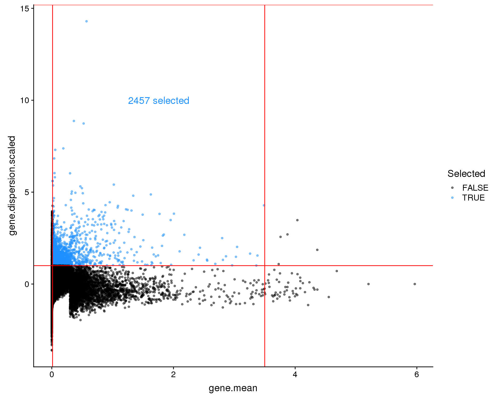
Expand here to see past versions of var-genes-1.png:
| Version | Author | Date |
|---|---|---|
| b8ba005 | Luke Zappia | 2019-02-24 |
| 8f826ef | Luke Zappia | 2019-02-08 |
| 2daa7f2 | Luke Zappia | 2019-01-25 |
| eaf03df | Luke Zappia | 2019-01-24 |
This approach has selected 2457 genes but it is difficult to know where to set the thresholds. Let’s have a look at another approach.
M3Drop
M3Drop implements an alternative approach that considers the expected number of zeros rather than gene dispersion. For UMI data a library-size adjusted negative binomial model is fitted and we look for genes that have more zeros than expected.
Fitting
DANB_fit  <- NBumiFitModel(seurat@raw.data)
fit_stats <- NBumiCheckFitFS(seurat@raw.data, DANB_fit, suppress.plot = TRUE)
names(fit_stats$rowPs) <- rownames(seurat@raw.data)
Comparison between fitted expected number of zeros and actual observed number of zeros.
Genes
plot_data <- tibble(
    Observed = DANB_fit$vals$djs,
    Fit = fit_stats$rowPs
)

ggplot(plot_data, aes(x = Observed, y = Fit)) +
    geom_point() +
    geom_abline(slope = 1, intercept = 0, colour = "red") +
    ggtitle("Gene dropout fit") +
    theme_minimal()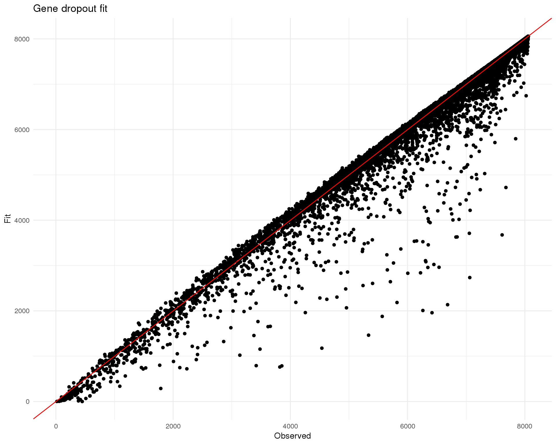
Cells
plot_data <- tibble(
    Observed = DANB_fit$vals$dis,
    Fit = fit_stats$colPs
)

ggplot(plot_data, aes(x = Observed, y = Fit)) +
    geom_point() +
    geom_abline(slope = 1, intercept = 0, colour = "red") +
    ggtitle("Cell dropout fit") +
    theme_minimal()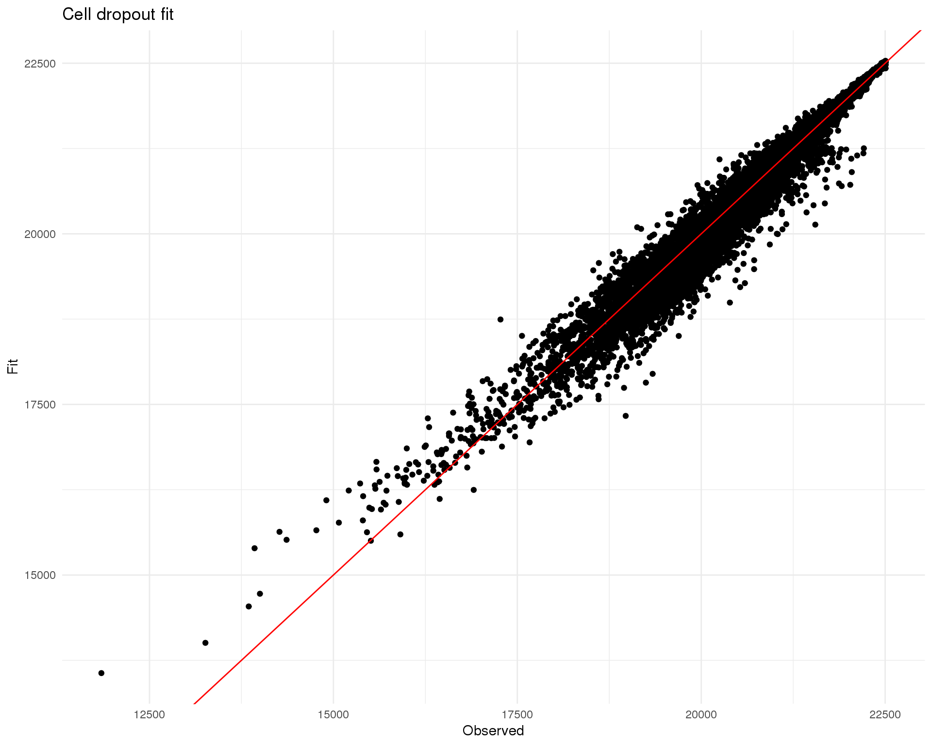
Selection
Selected genes are those that have significantly more zeros than expected based on the fitted distribution. This plot shows all of the genes in the dataset (light points coloured according to local density), selected genes (dark, outlined points) and the fitted distribution (red line).
m3drop_q <- 0.01

drop_features <- NBumiFeatureSelectionCombinedDrop(DANB_fit,
                                                   method = "fdr",
                                                   qval.thres = 1,
                                                   suppress.plot = TRUE) %>%
    mutate(Gene = as.character(Gene))

m3drop_results <- tibble(
    Gene = names(DANB_fit$sizes),
    AvgExpr = log10(DANB_fit$vals$tjs / DANB_fit$vals$nc),
    DropoutRate = DANB_fit$vals$djs / DANB_fit$vals$nc
) %>%
    mutate(DensCol = densCols(AvgExpr, DropoutRate, colramp = viridis)) %>%
    mutate(DropoutExp = fit_stats$rowPs[Gene] / DANB_fit$vals$nc) %>%
    left_join(drop_features, by = "Gene")

m3drop_top <- filter(m3drop_results, q.value < m3drop_q)

ggplot(m3drop_results) +
    geom_point(aes(x = AvgExpr, y = DropoutRate,
                   colour = colorspace::lighten(DensCol, amount = 0.4))) +
    scale_colour_identity() +
    geom_point(data = m3drop_top,
               aes(x = AvgExpr, y = DropoutRate, fill = DensCol),
               colour = "dodgerblue", shape = 21) +
    scale_fill_identity() +
    geom_line(aes(x = AvgExpr, y = DropoutExp), colour = "red") +
    xlab("log10(average expression)") +
    ylab("Dropout rate") +
    theme_minimal()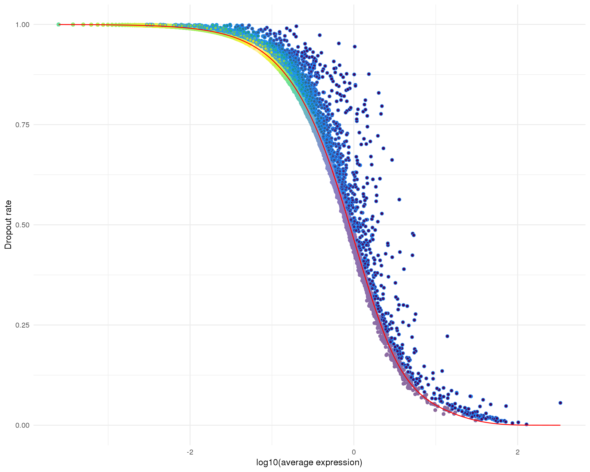
Expand here to see past versions of m3drop-select-1.png:
| Version | Author | Date |
|---|---|---|
| b8ba005 | Luke Zappia | 2019-02-24 |
| 8f826ef | Luke Zappia | 2019-02-08 |
| 2daa7f2 | Luke Zappia | 2019-01-25 |
| eaf03df | Luke Zappia | 2019-01-24 |
This method identifies 1952 genes.
Comparison
seurat_hvg                    <- seurat@hvg.info[rownames(sce), ]
rowData(sce)$SeuratMean       <- seurat_hvg$gene.mean
rowData(sce)$SeuratDisp       <- seurat_hvg$gene.dispersion
rowData(sce)$SeuratDispScaled <- seurat_hvg$gene.dispersion.scaled
rowData(sce)$SeuratSelected   <- rownames(sce) %in% seurat@var.genes

rowData(sce)$M3DropAvgExpr     <- m3drop_results$AvgExpr
rowData(sce)$M3DropDropoutRate <- m3drop_results$DropoutRate
rowData(sce)$M3DropDropoutExp  <- m3drop_results$DropoutExp
rowData(sce)$M3DropEffect      <- m3drop_results$effect_size
rowData(sce)$M3DropPValue      <- m3drop_results$p.value
rowData(sce)$M3DropFDR         <- m3drop_results$q.value
rowData(sce)$M3DropSelected    <- rownames(sce) %in% m3drop_top$Gene

rowData(sce)$SelMethod <- "False"
rowData(sce)$SelMethod[rowData(sce)$SeuratSelected] <- "Seurat only"
rowData(sce)$SelMethod[rowData(sce)$M3DropSelected] <- "M3Drop only"
rowData(sce)$SelMethod[rowData(sce)$SeuratSelected &
                           rowData(sce)$M3DropSelected] <- "Both"

plot_data <- rowData(sce) %>%
    as.data.frame() %>%
    select(SeuratMean, SeuratDispScaled, M3DropAvgExpr, M3DropDropoutRate,
           SelMethod)

plot_data_sel <- plot_data %>%
    filter(SelMethod != "False")
Let’s briefly compare the results from the two methods.
Number
Number of genes identified by each method.
ggplot(plot_data_sel, aes(x = SelMethod, fill = SelMethod)) +
    geom_bar() +
    theme_minimal() +
    theme(legend.position = "none",
          axis.title = element_blank())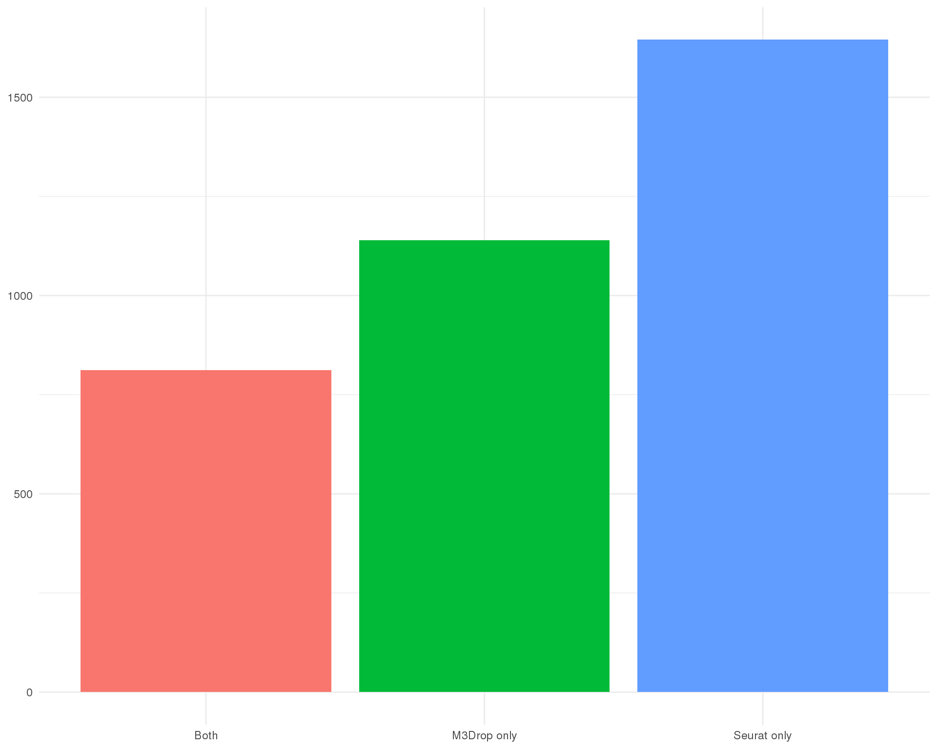
Seurat
Seurat selection plot coloured by selection method.
ggplot(plot_data, aes(x = SeuratMean, y = SeuratDispScaled)) +
    geom_point(alpha = 0.5, colour = "grey") +
    geom_point(data = plot_data_sel, aes(colour = SelMethod)) +
    theme_minimal()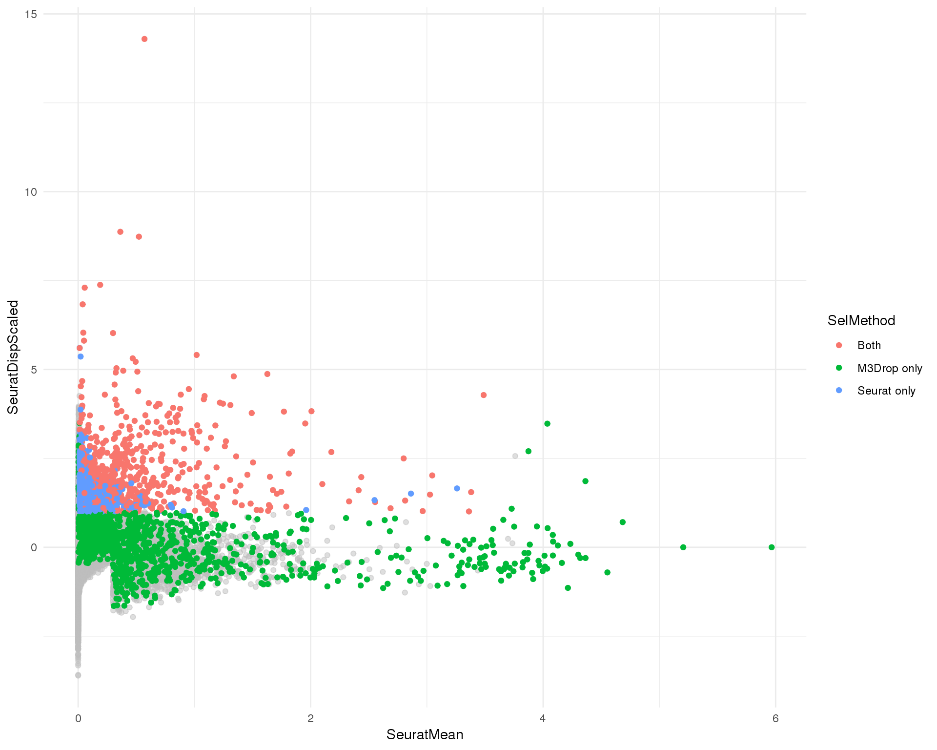
M3Drop
M3Drop selection plot coloured by selection method.
ggplot(plot_data, aes(x = M3DropAvgExpr, y = M3DropDropoutRate)) +
    geom_point(alpha = 0.5, colour = "grey") +
    geom_point(data = plot_data_sel, aes(colour = SelMethod)) +
    theme_minimal()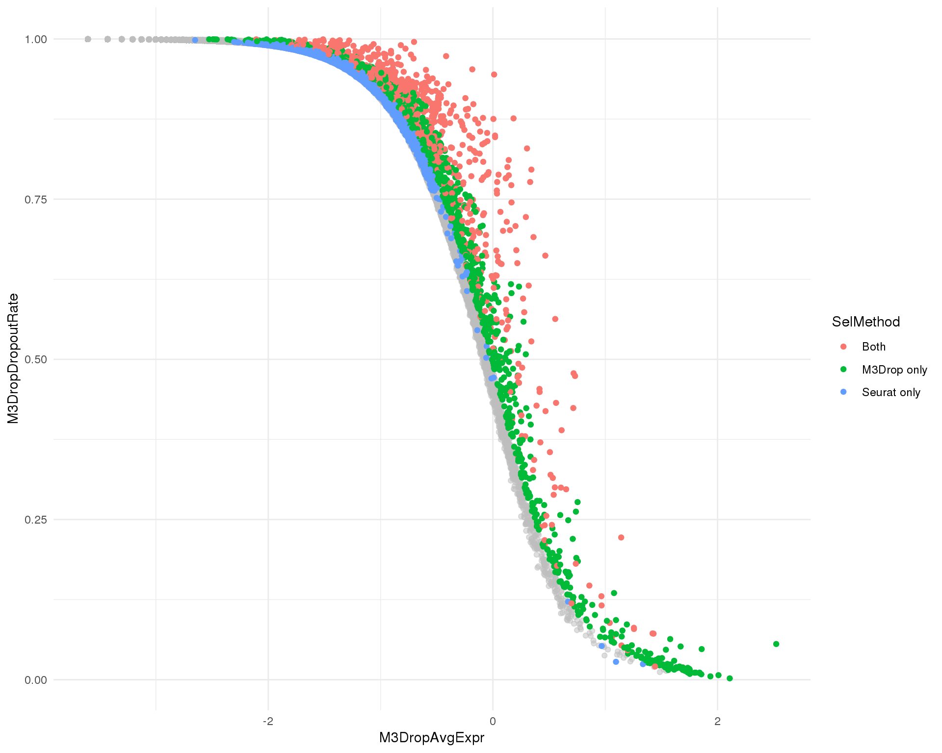
Combined
M3Drop dropout rate against Seurat dispersion coloured by selection method.
ggplot(plot_data, aes(x = SeuratDispScaled, y = M3DropDropoutRate)) +
    geom_point(alpha = 0.5, colour = "grey") +
    geom_point(data = plot_data_sel, aes(colour = SelMethod)) +
    theme_minimal()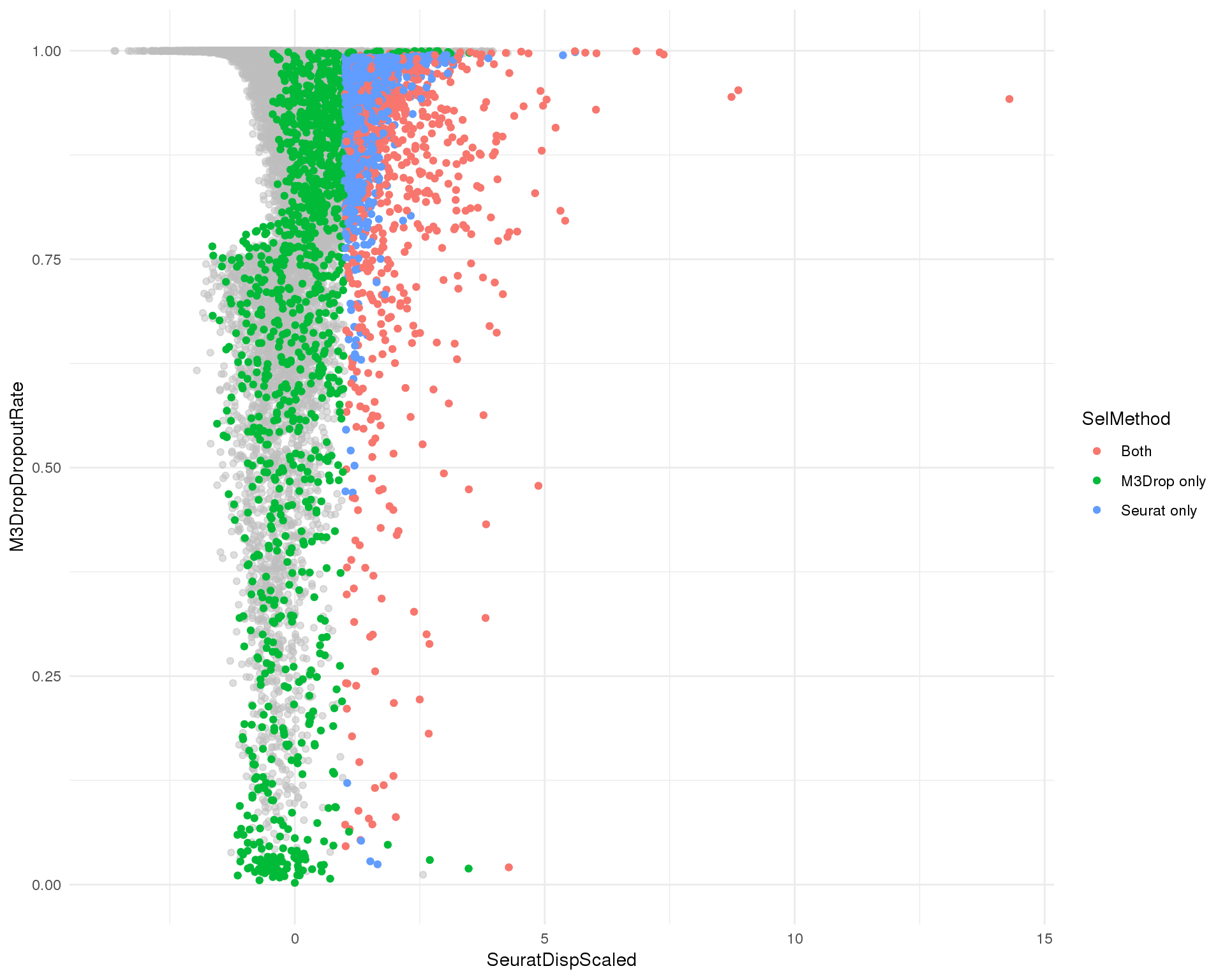
PCA (Seurat)
PCA of cells using genes selected by the Seurat method.
seurat <- RunPCA(seurat, pc.genes = seurat@var.genes, pcs.compute = 2,
                 do.print = FALSE, reduction.name = "pca_seurat")

ggplot(as.data.frame(seurat@dr$pca_seurat@cell.embeddings),
       aes(x = PC1, y = PC2)) +
    geom_point(alpha = 0.5, colour = "grey20") +
    theme_minimal()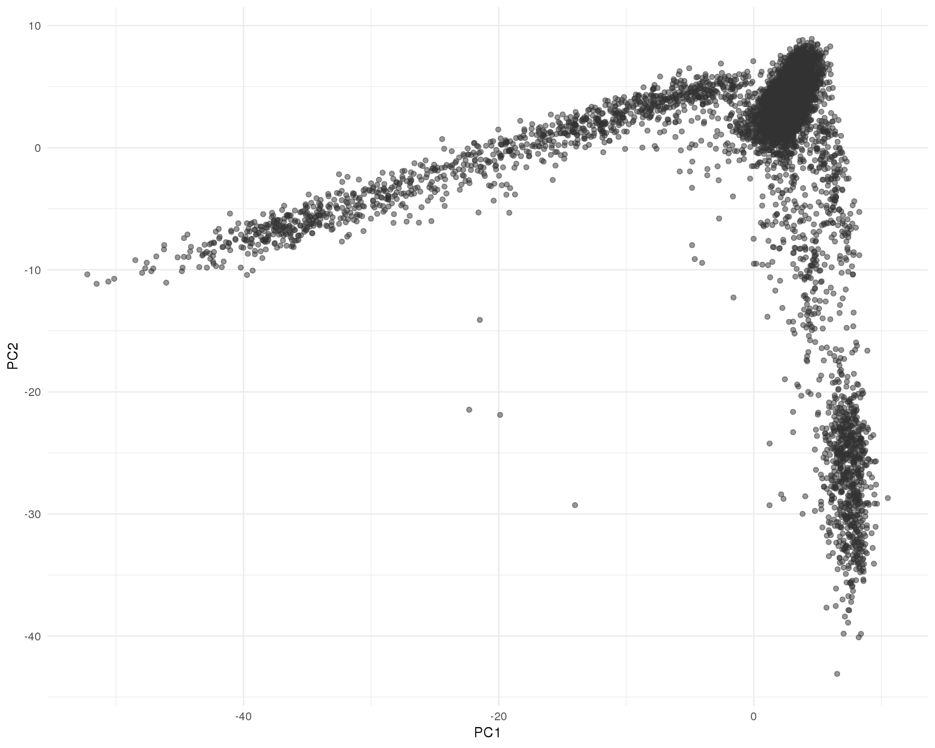
PCA (M3Drop)
PCA of cells using genes selected by the M3Drop method.
seurat <- RunPCA(seurat, pc.genes = m3drop_top$Gene, pcs.compute = 2,
                 do.print = FALSE, reduction.name = "pca_m3drop")

ggplot(as.data.frame(seurat@dr$pca_m3drop@cell.embeddings),
       aes(x = PC1, y = PC2)) +
    geom_point(alpha = 0.5, colour = "grey20") +
    theme_minimal()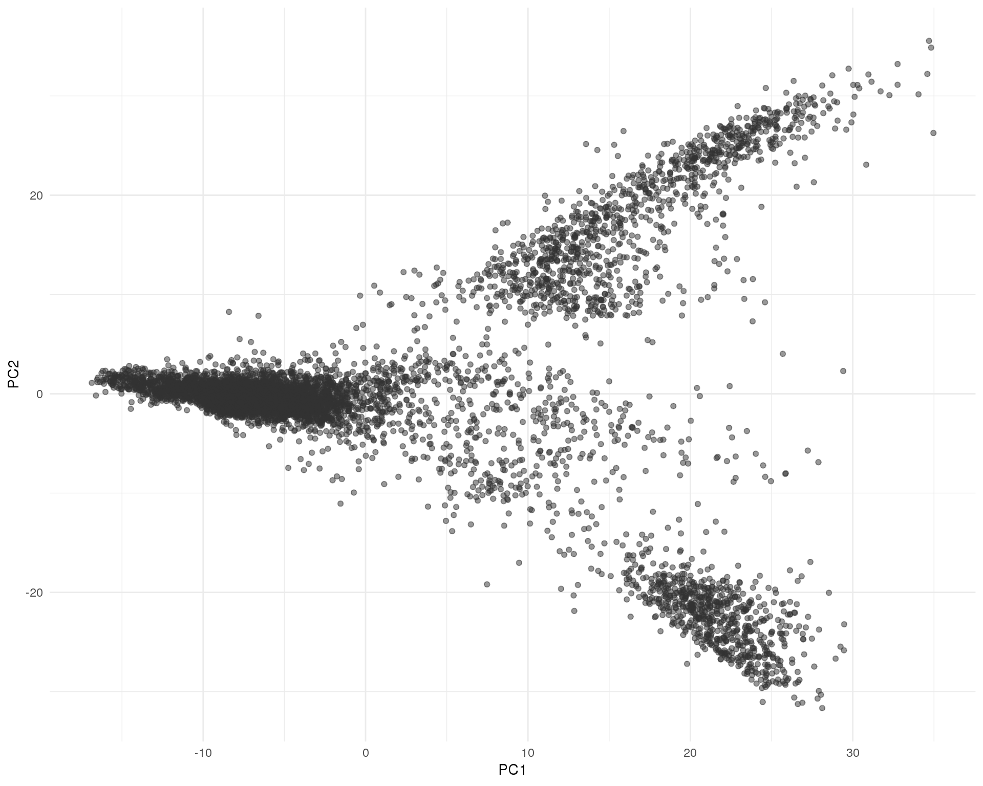
Selection
For the rest of the analysis we will use the M3Drop genes.
rowData(sce)$Selected <- rowData(sce)$M3DropSelected
seurat@var.genes <- m3drop_top$Gene

sel_genes <- rowData(sce) %>%
    as.data.frame() %>%
    filter(Selected) %>%
    select(Name, ID, entrezgene, description, starts_with("M3Drop"),
           -M3DropSelected) %>%
    arrange(-M3DropEffect)

sel_genes
Dimensionality reduction
The next step in the Seurat workflow is to select a set of principal components that capture the variance in the dataset using the selected genes.
seurat <- RunPCA(seurat, pc.genes = seurat@var.genes, pcs.compute = 50,
                 do.print = FALSE)
These plots show the genes and variance associated with the principal components and help use to select how many to use.
Plots
Elbow
Variance explained by each principal component.
PCElbowPlot(seurat, num.pc = 50)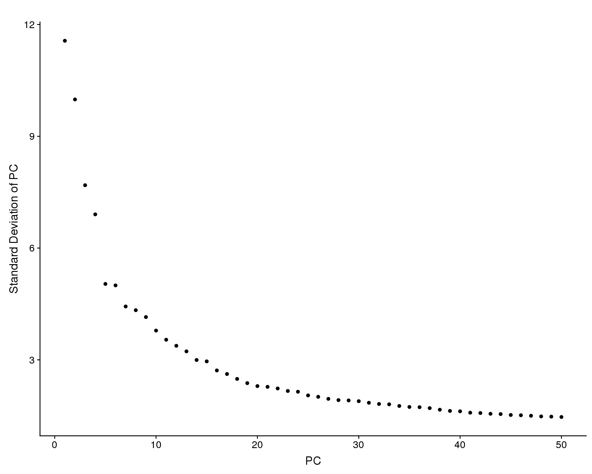
Gene loadings
PCA loadings of genes associated with some principal components.
VizPCA(seurat, pcs.use = 1:9, num.genes = 20, font.size = 1)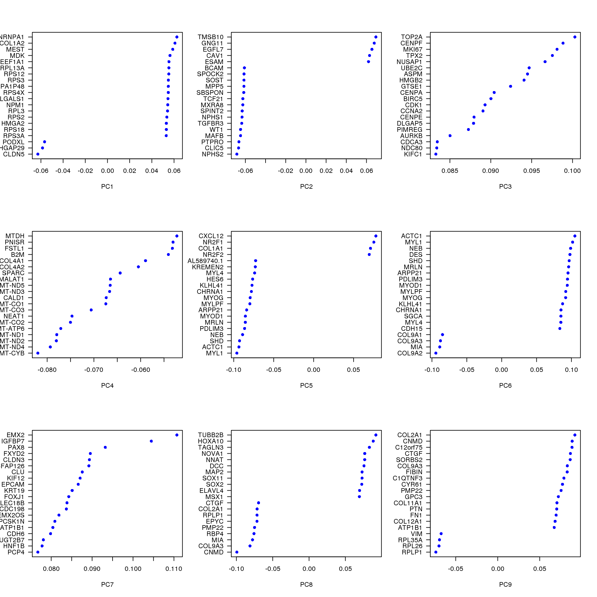
Heatmap
Heatmap of genes associated with some principal components.
PCHeatmap(object = seurat, pc.use = 1:9, cells.use = 500, do.balanced = TRUE,
          label.columns = FALSE)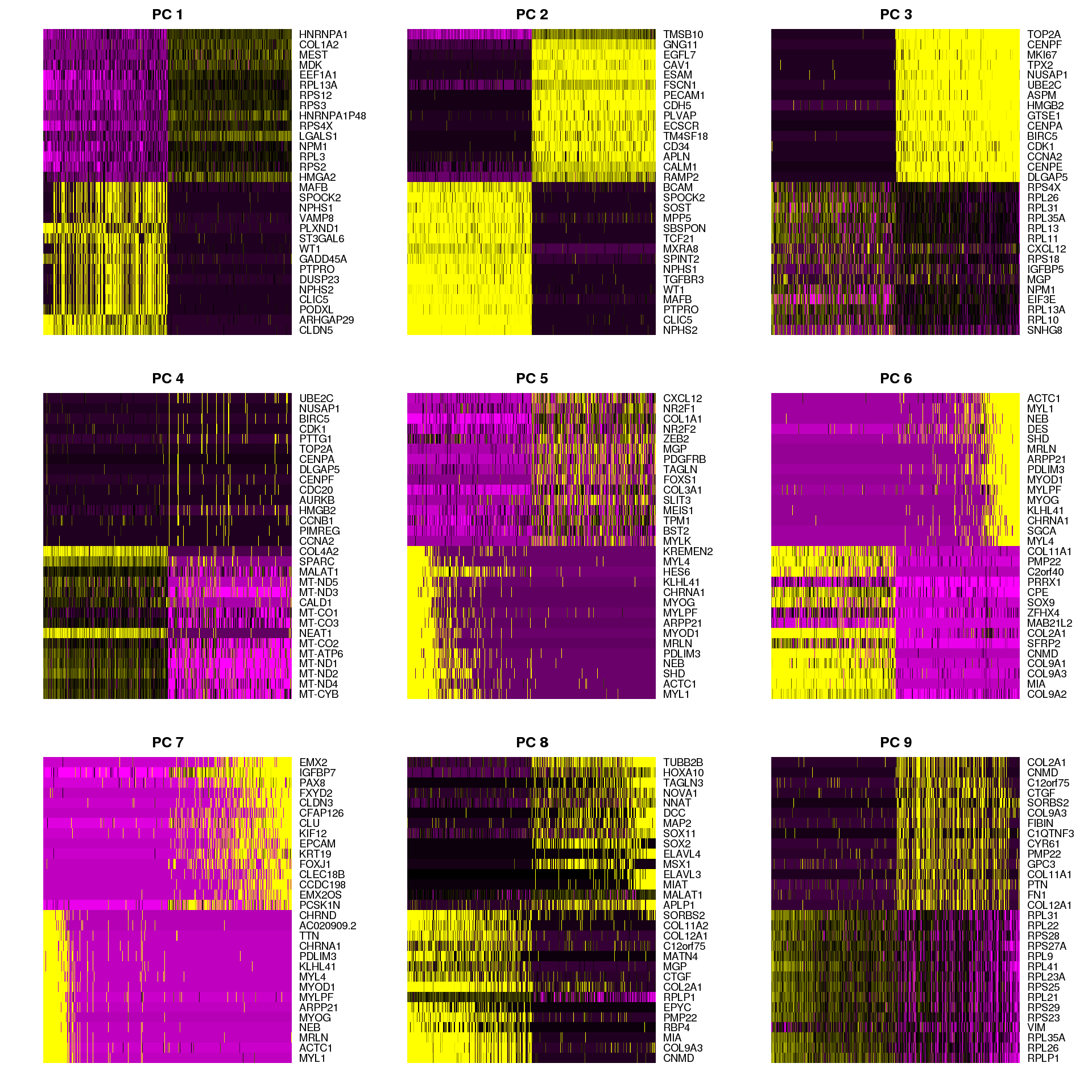
Selection
n_pcs <- 15
seurat <- RunTSNE(seurat, dims.use = 1:n_pcs)
Based on these plots we will use the first 15 principal components.
Resolution
Now that we have a set of principal components we can perform clustering. Seurat uses a graph-based clustering method which has a resolution parameter that controls the number of clusters that are produced. We are going to cluster at a range of resolutions and select one that gives a reasonable division of this dataset.
resolutions <- seq(0, 1, 0.1)
knn <- 30

seurat <- FindClusters(seurat,
                       reduction.type = "pca", dims.use = 1:n_pcs,
                       k.param = knn,
                       resolution = resolutions,
                       save.SNN = TRUE,
                       print.output = FALSE)
Dimensionlity reduction
Dimensionality reduction plots showing clusters at different resolutions.
PCA
src_list <- lapply(resolutions, function(res) {
    src <- c(
        "#### Res {{res}} {.unnumbered}",
        "```{r res-pca-{{res}}}",
        "PCAPlot(seurat, group.by = 'res.{{res}}', do.label = TRUE)",
        "```",
        ""
    )
    knit_expand(text = src)
})

out <- knit_child(text = unlist(src_list), options = list(cache = FALSE))
Res 0
PCAPlot(seurat, group.by = 'res.0', do.label = TRUE)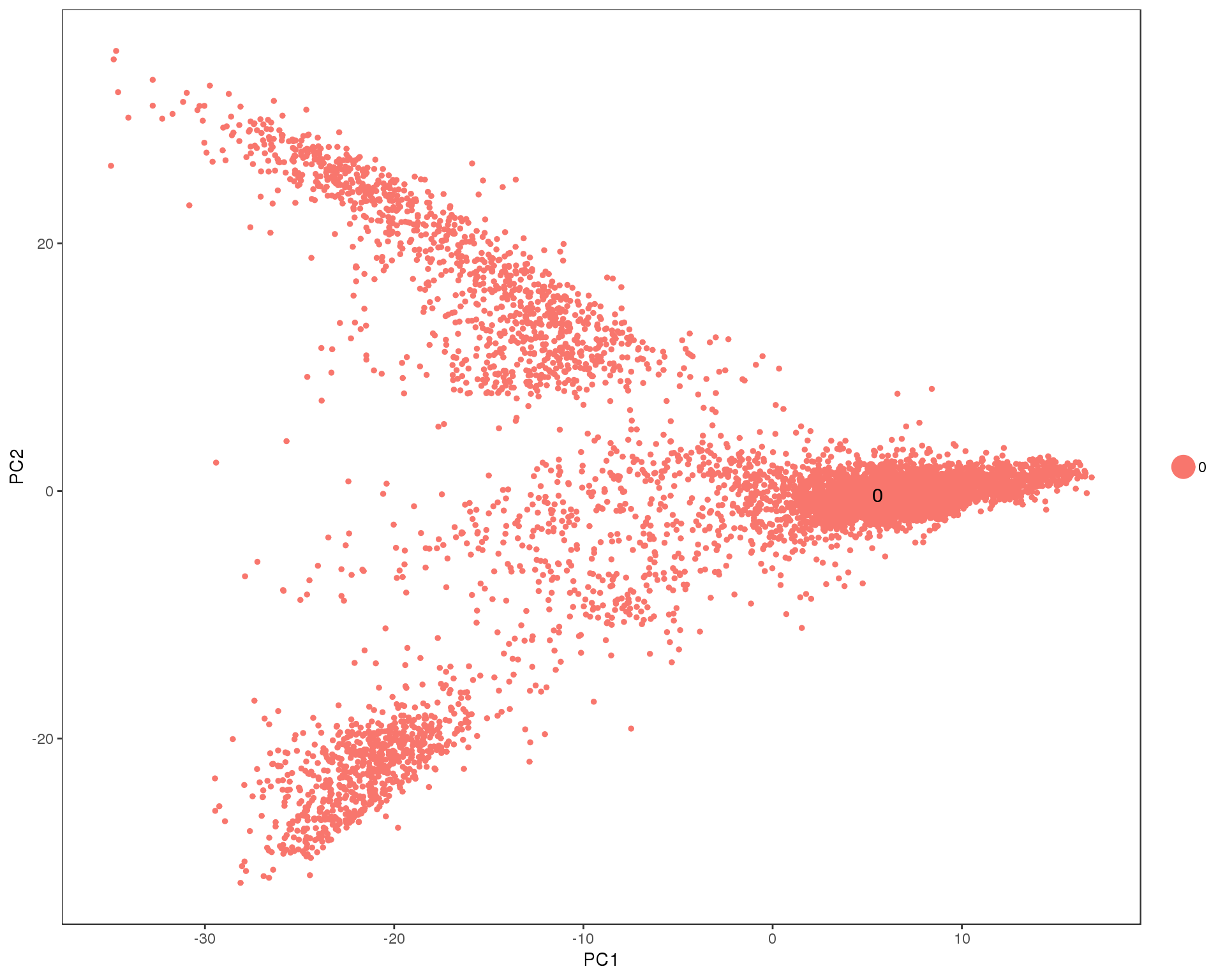
Res 0.1
PCAPlot(seurat, group.by = 'res.0.1', do.label = TRUE)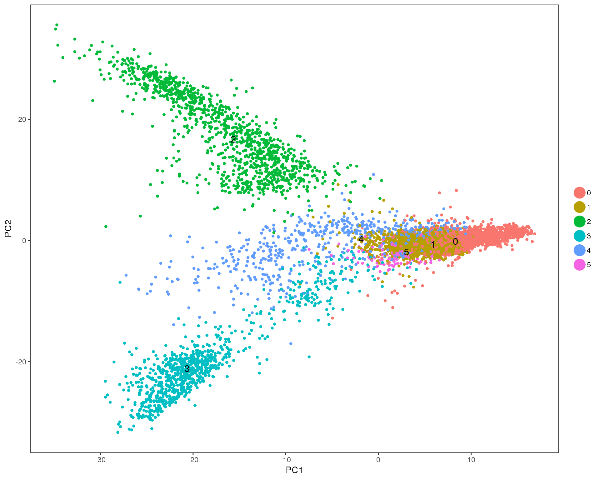
Res 0.2
PCAPlot(seurat, group.by = 'res.0.2', do.label = TRUE)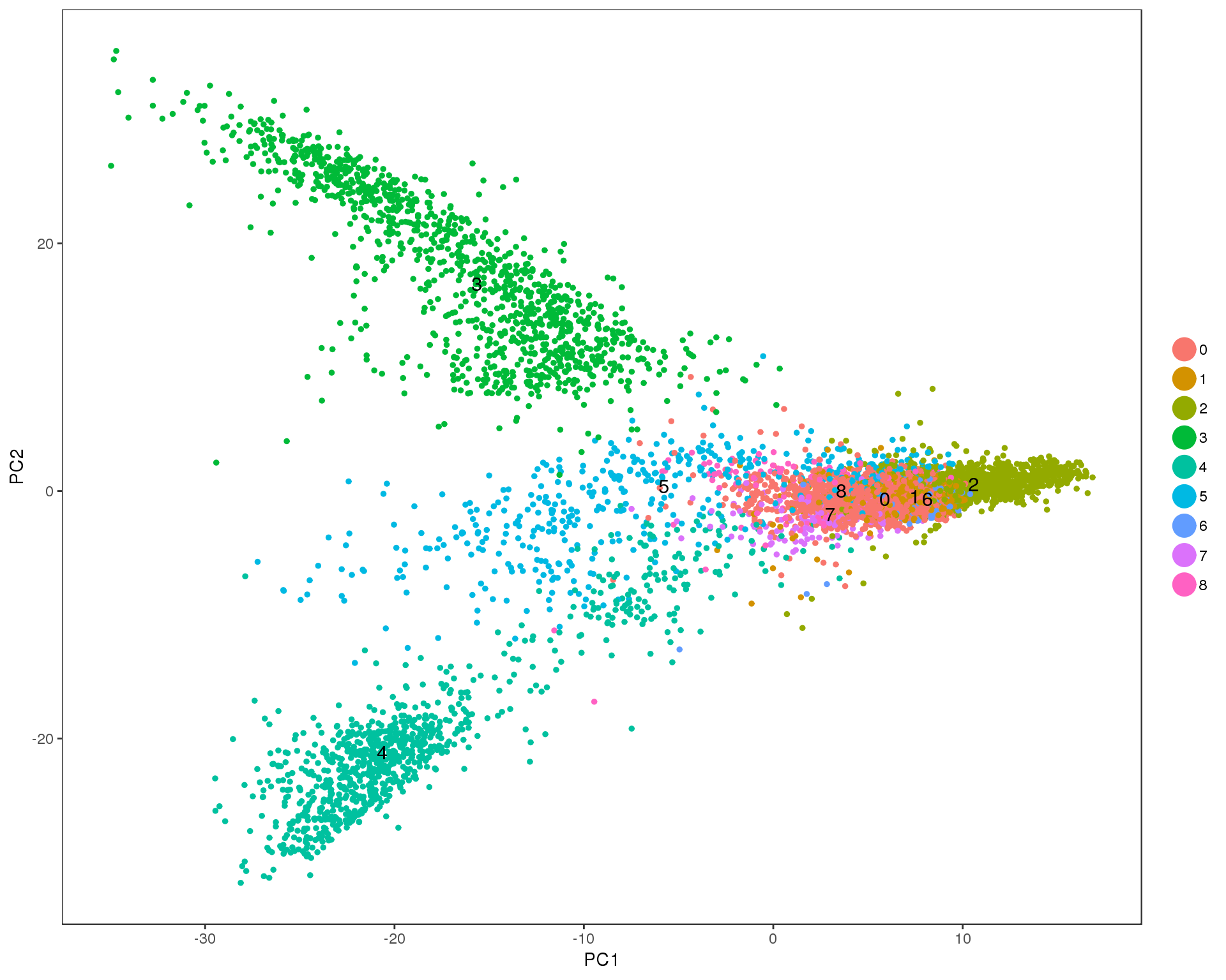
Res 0.3
PCAPlot(seurat, group.by = 'res.0.3', do.label = TRUE)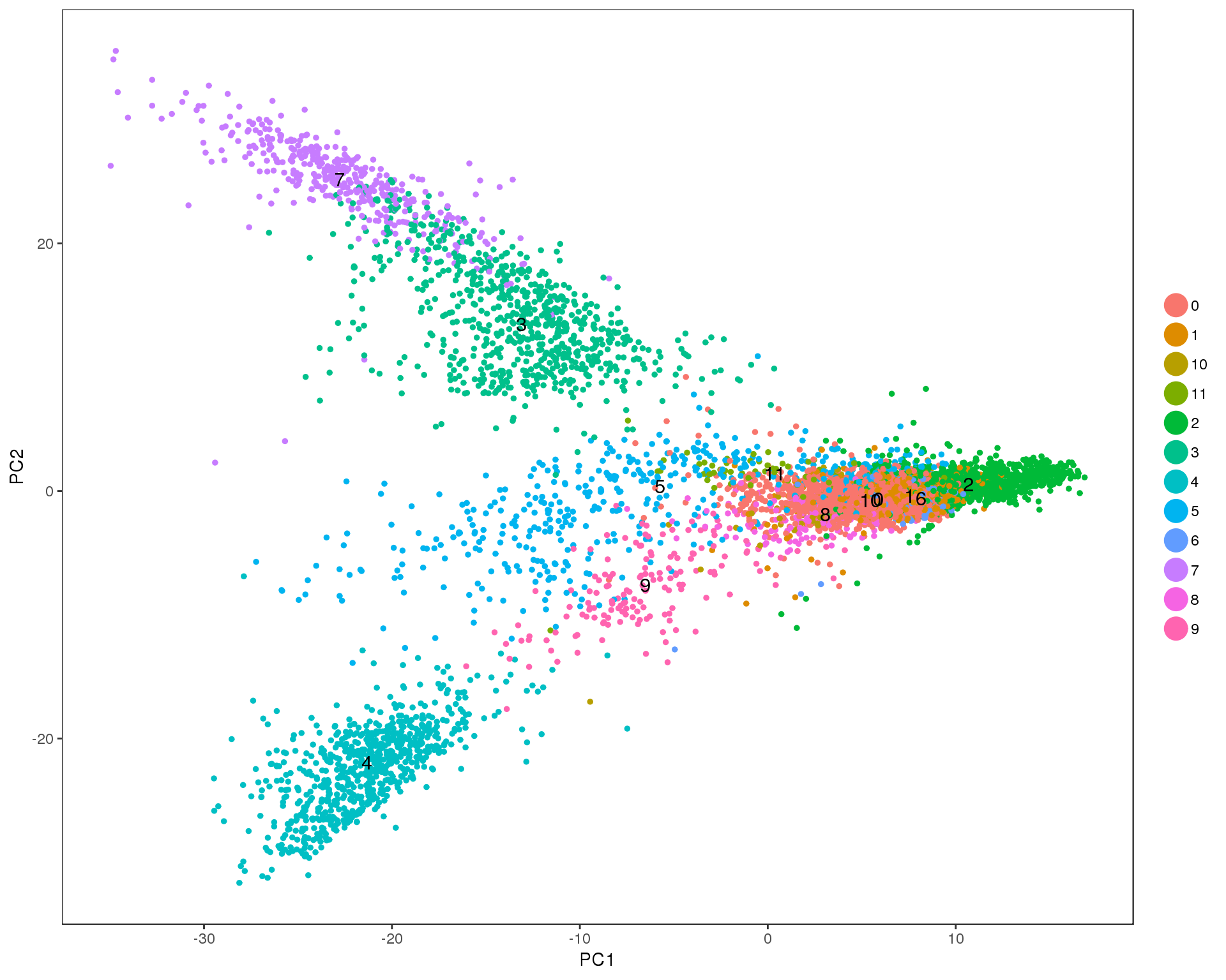
Res 0.4
PCAPlot(seurat, group.by = 'res.0.4', do.label = TRUE)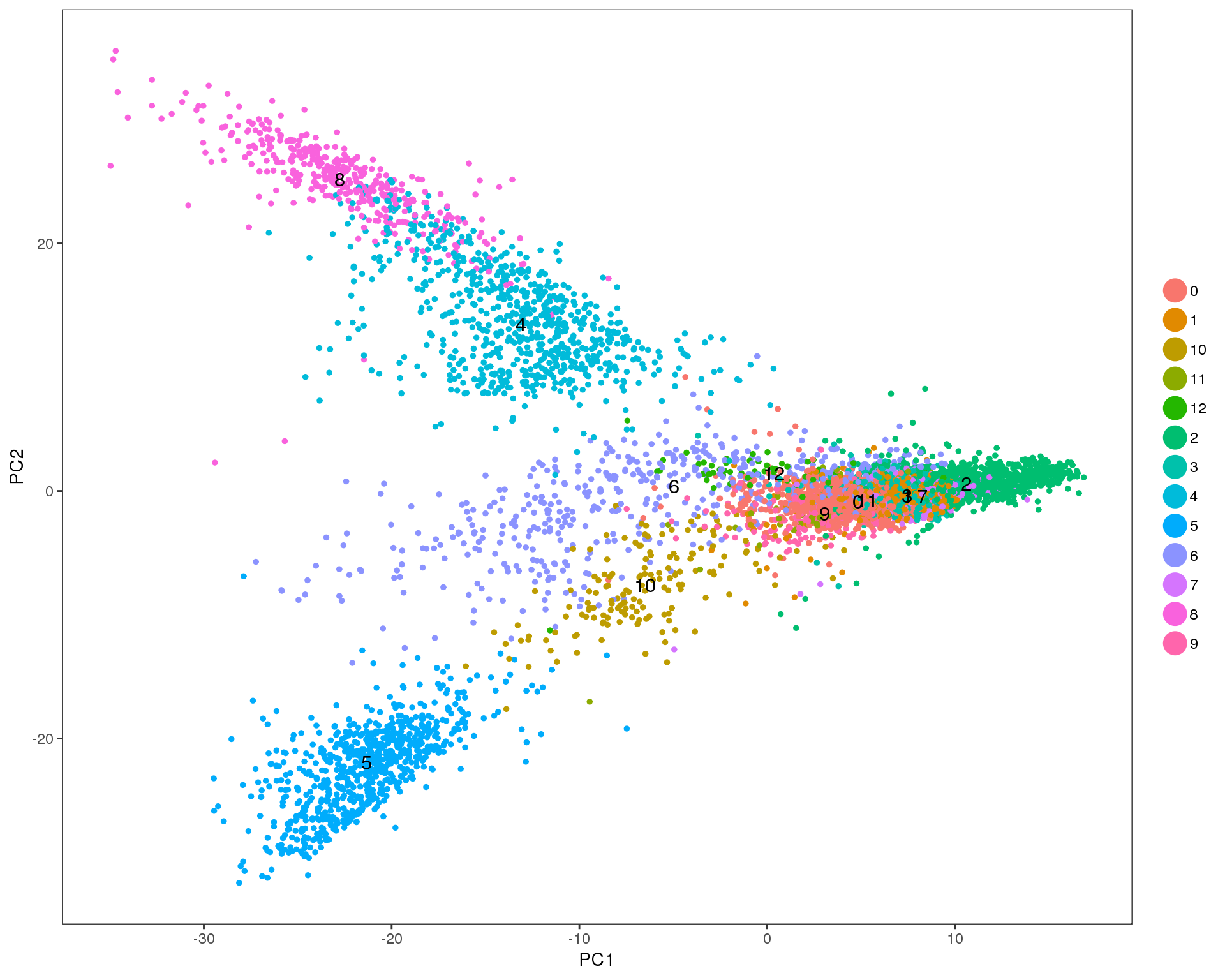
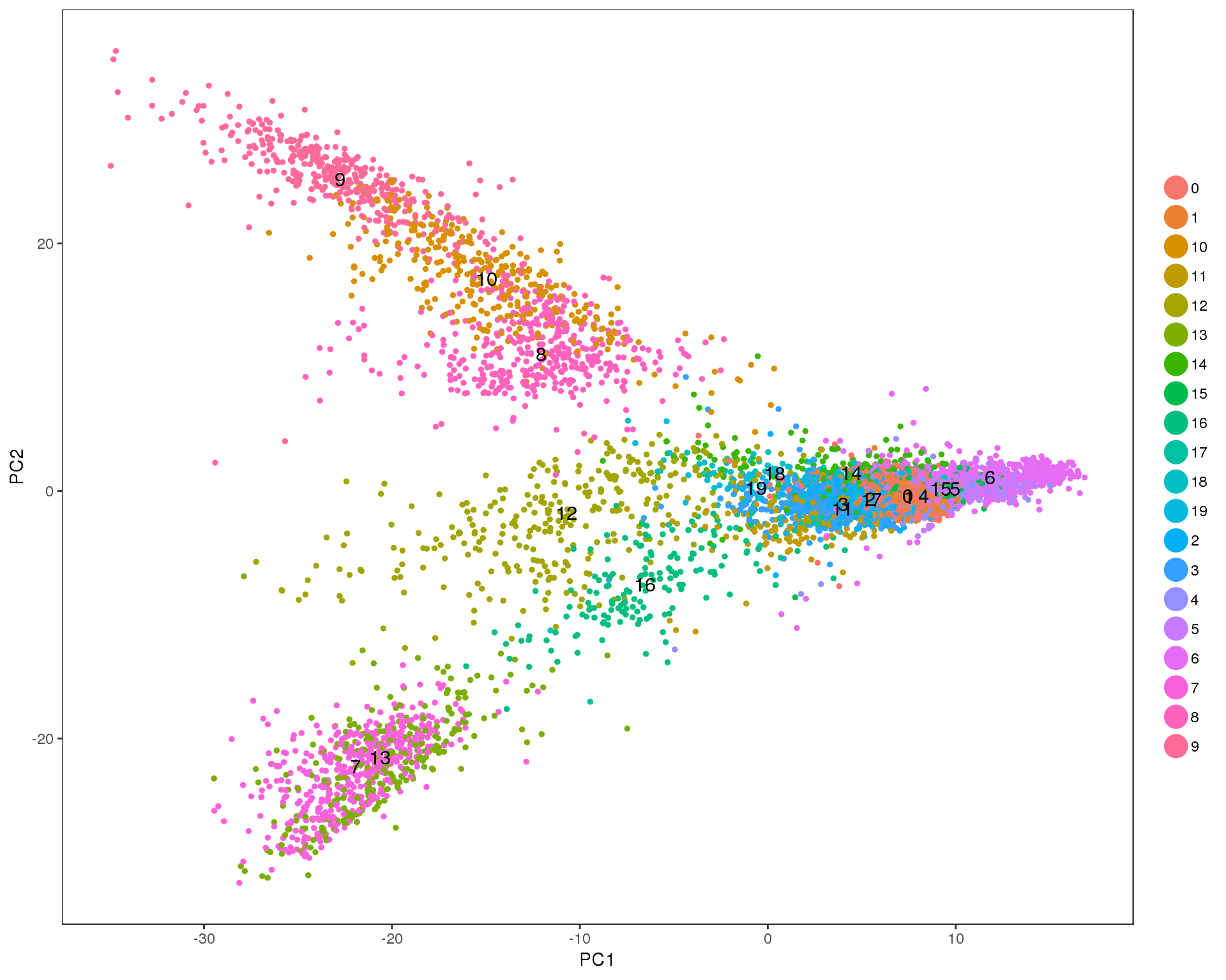
Res 0.5
PCAPlot(seurat, group.by = 'res.0.5', do.label = TRUE)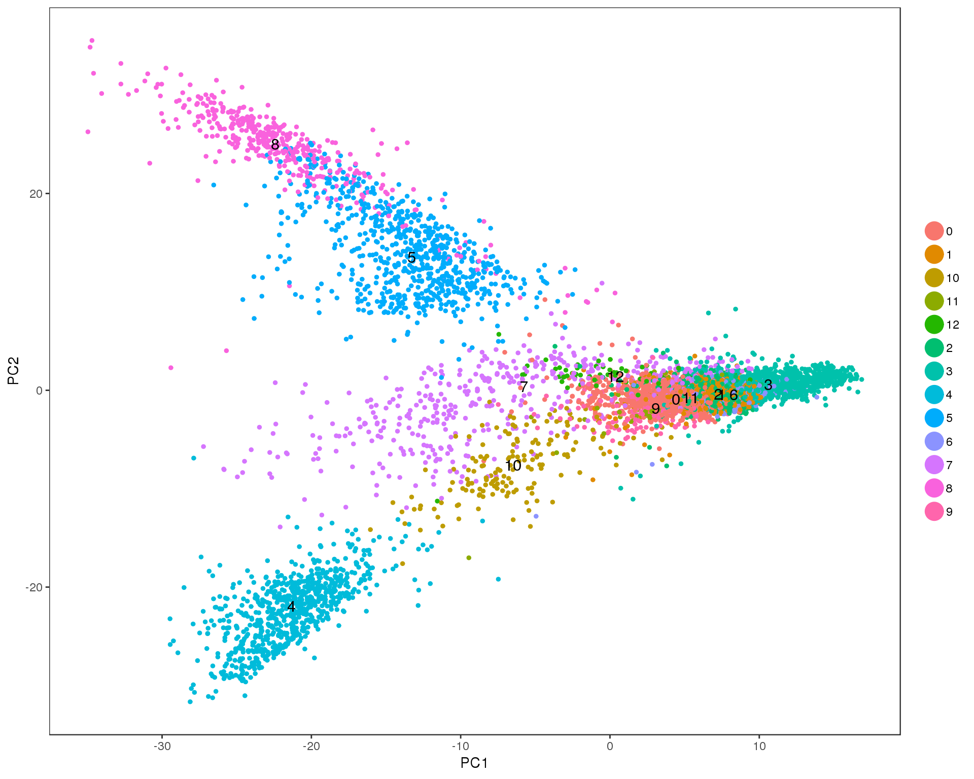
Res 0.6
PCAPlot(seurat, group.by = 'res.0.6', do.label = TRUE)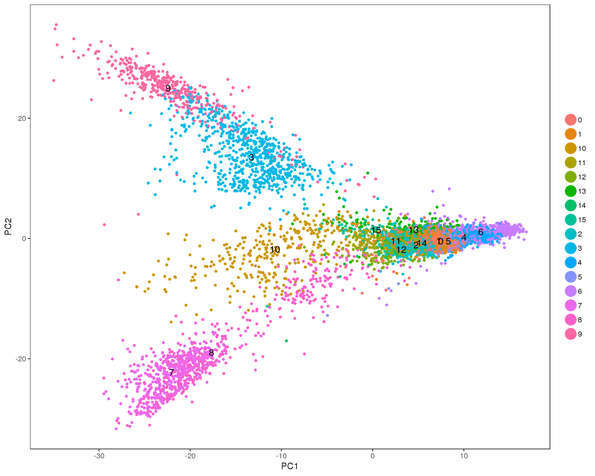
Res 0.7
PCAPlot(seurat, group.by = 'res.0.7', do.label = TRUE)
Res 0.8
PCAPlot(seurat, group.by = 'res.0.8', do.label = TRUE)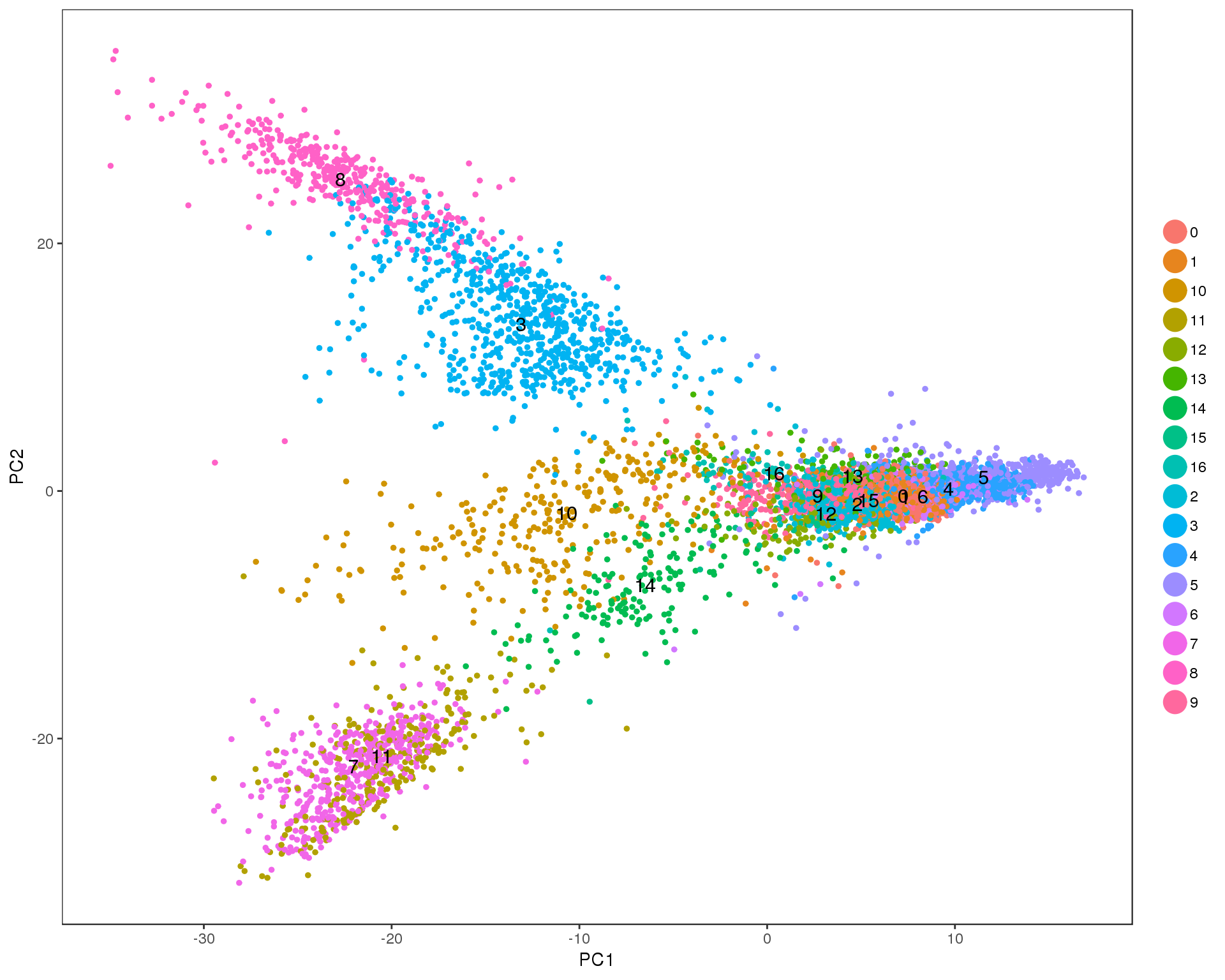
Res 0.9
PCAPlot(seurat, group.by = 'res.0.9', do.label = TRUE)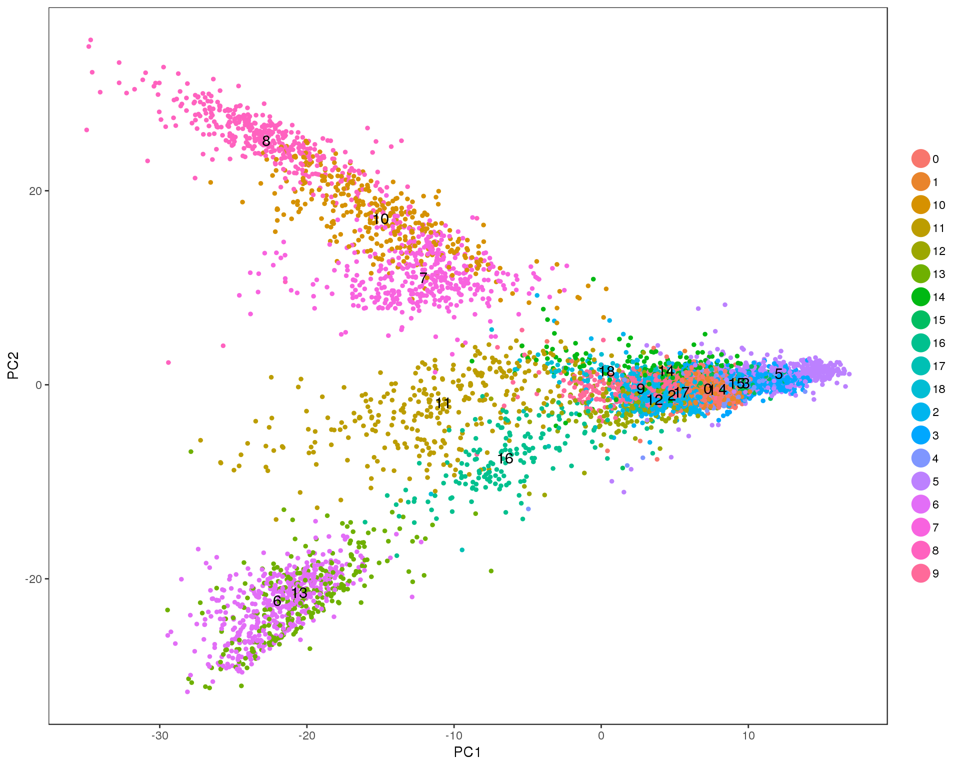
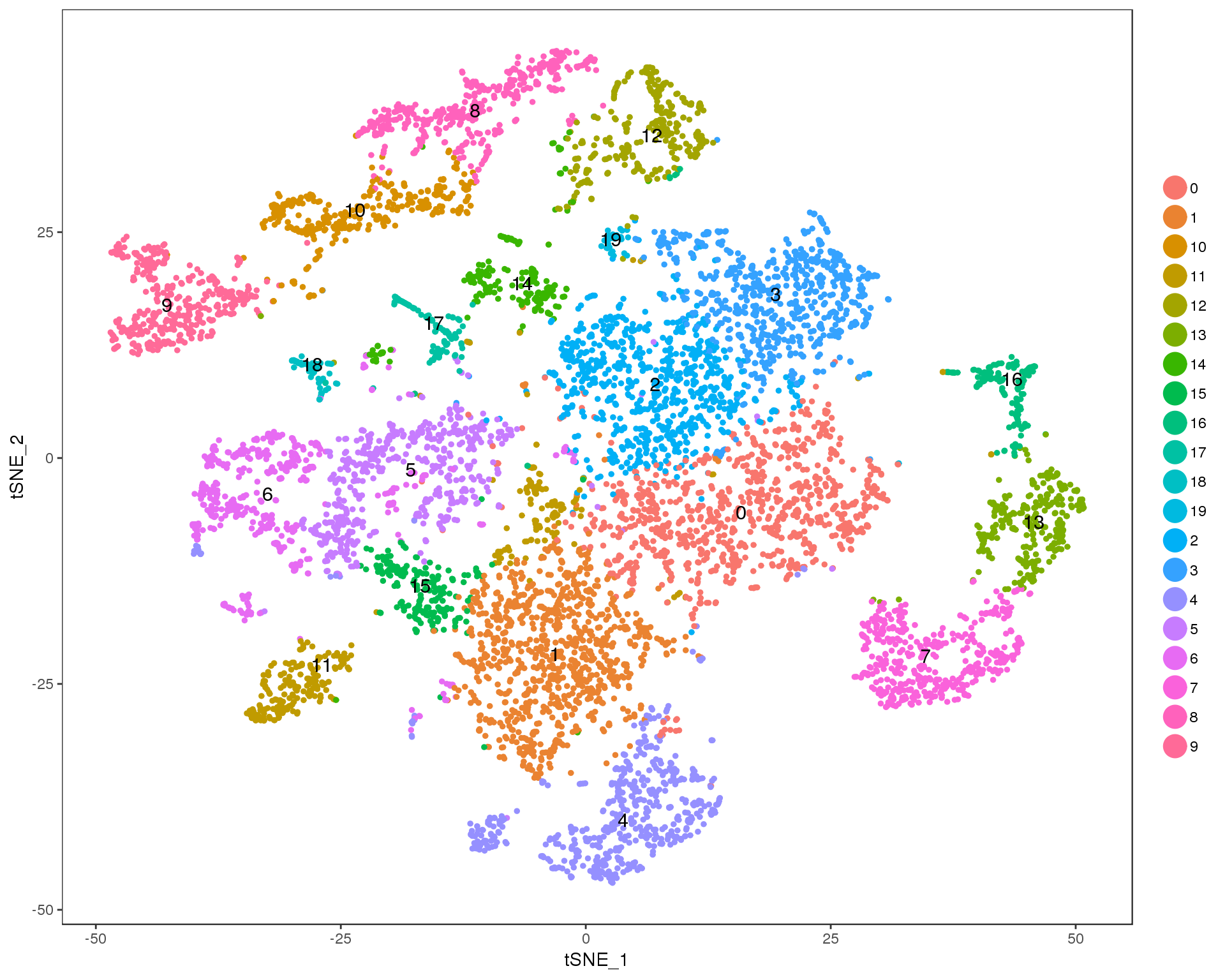
t-SNE
src_list <- lapply(resolutions, function(res) {
    src <- c(
        "#### Res {{res}} {.unnumbered}",
        "```{r res-tSNE-{{res}}}",
        "TSNEPlot(seurat, group.by = 'res.{{res}}', do.label = TRUE)",
        "```",
        ""
    )
    knit_expand(text = src)
})

out <- knit_child(text = unlist(src_list), options = list(cache = FALSE))
Res 0
TSNEPlot(seurat, group.by = 'res.0', do.label = TRUE)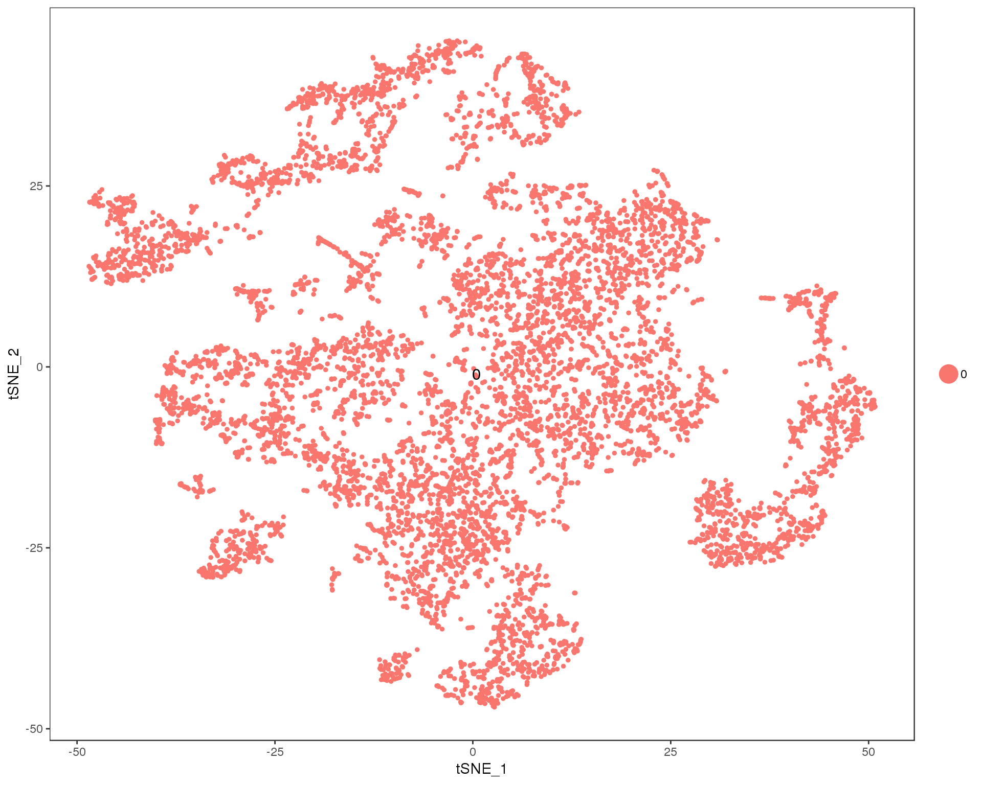
Res 0.1
TSNEPlot(seurat, group.by = 'res.0.1', do.label = TRUE)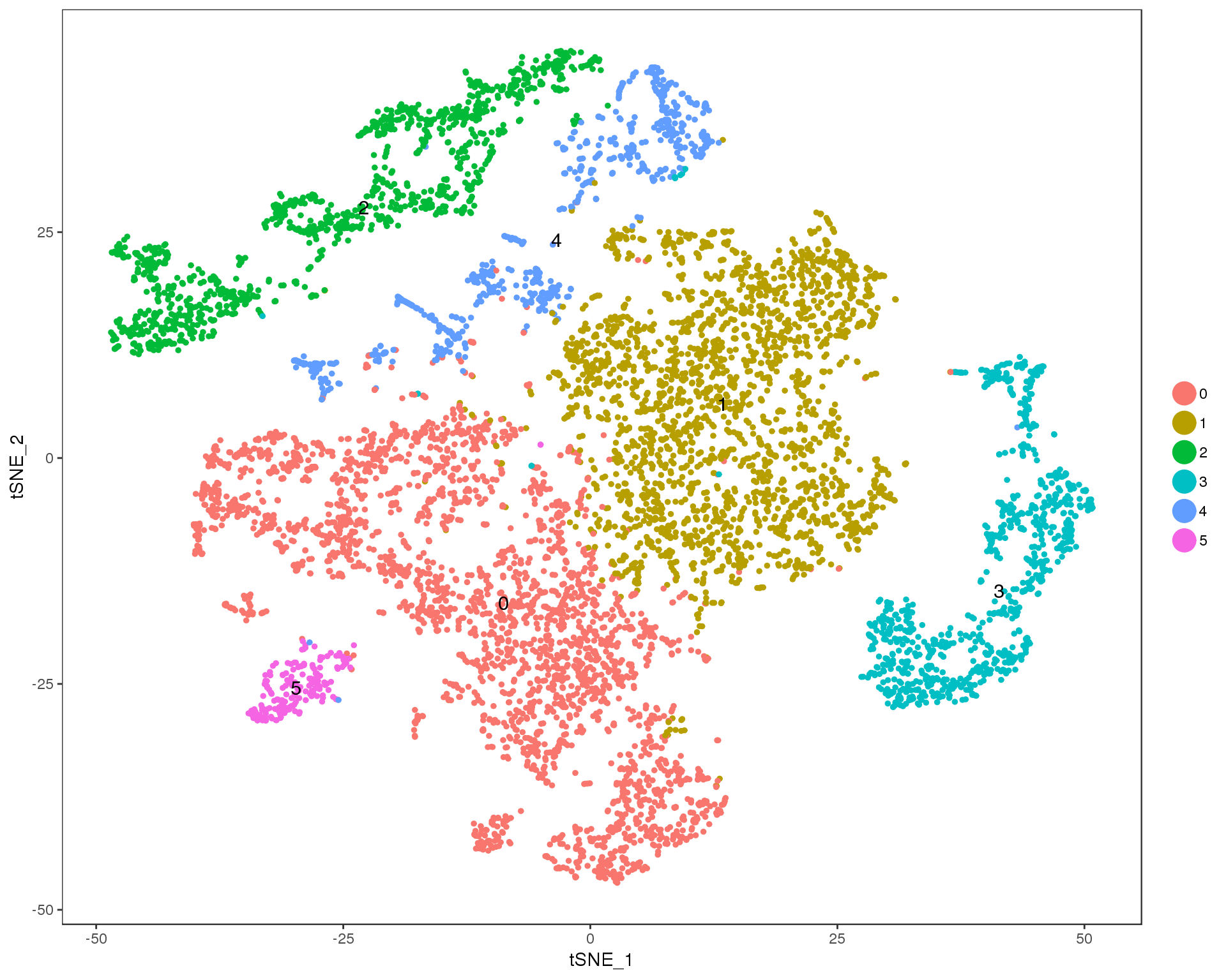
Res 0.2
TSNEPlot(seurat, group.by = 'res.0.2', do.label = TRUE)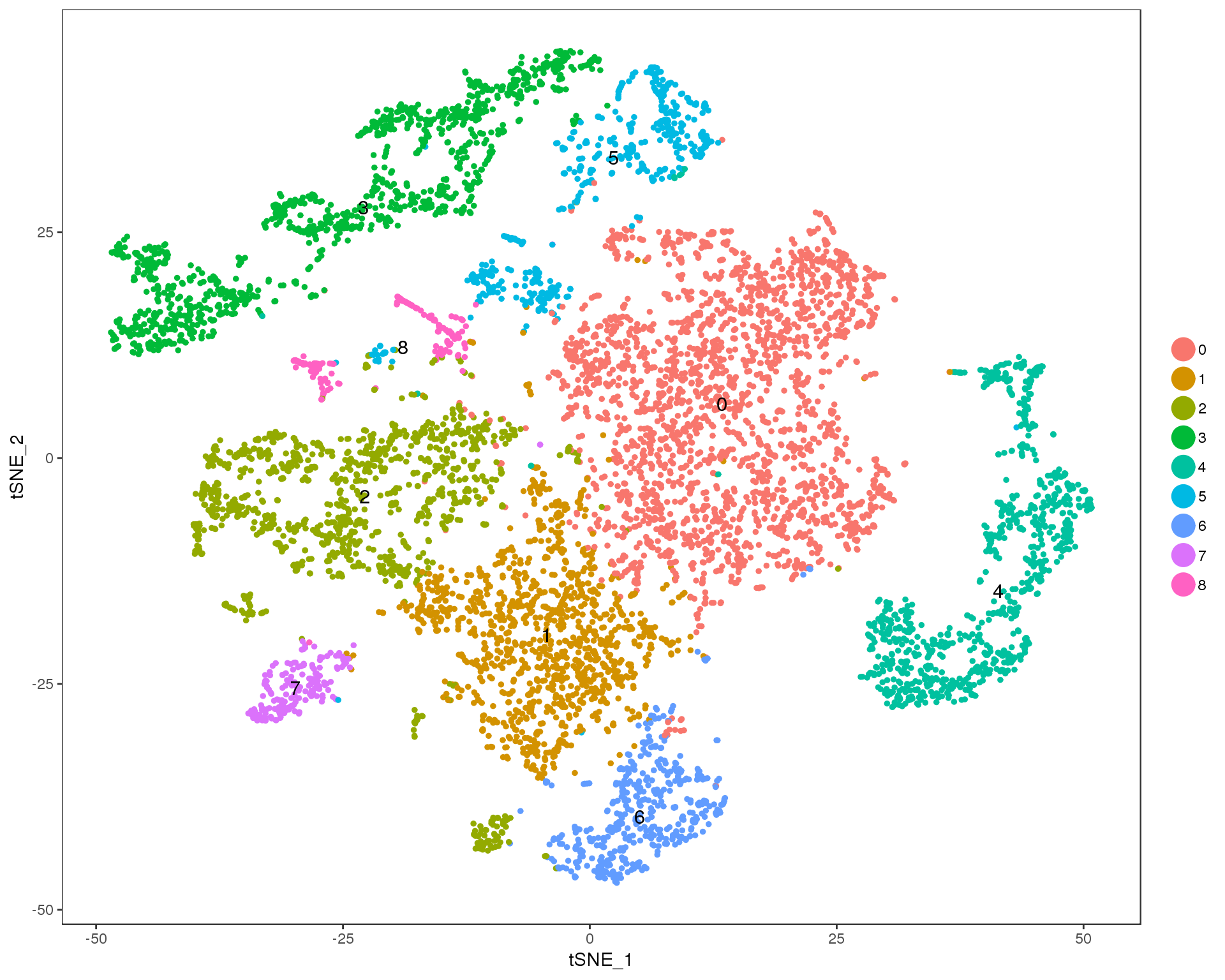
Res 0.3
TSNEPlot(seurat, group.by = 'res.0.3', do.label = TRUE)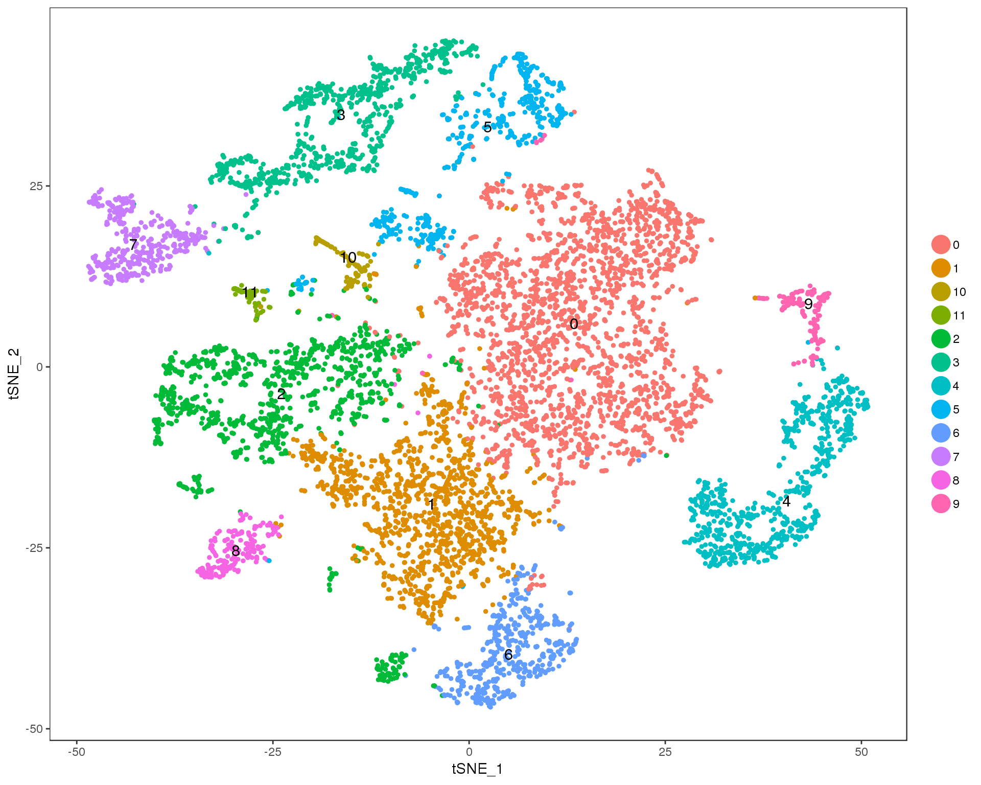
Res 0.4
TSNEPlot(seurat, group.by = 'res.0.4', do.label = TRUE)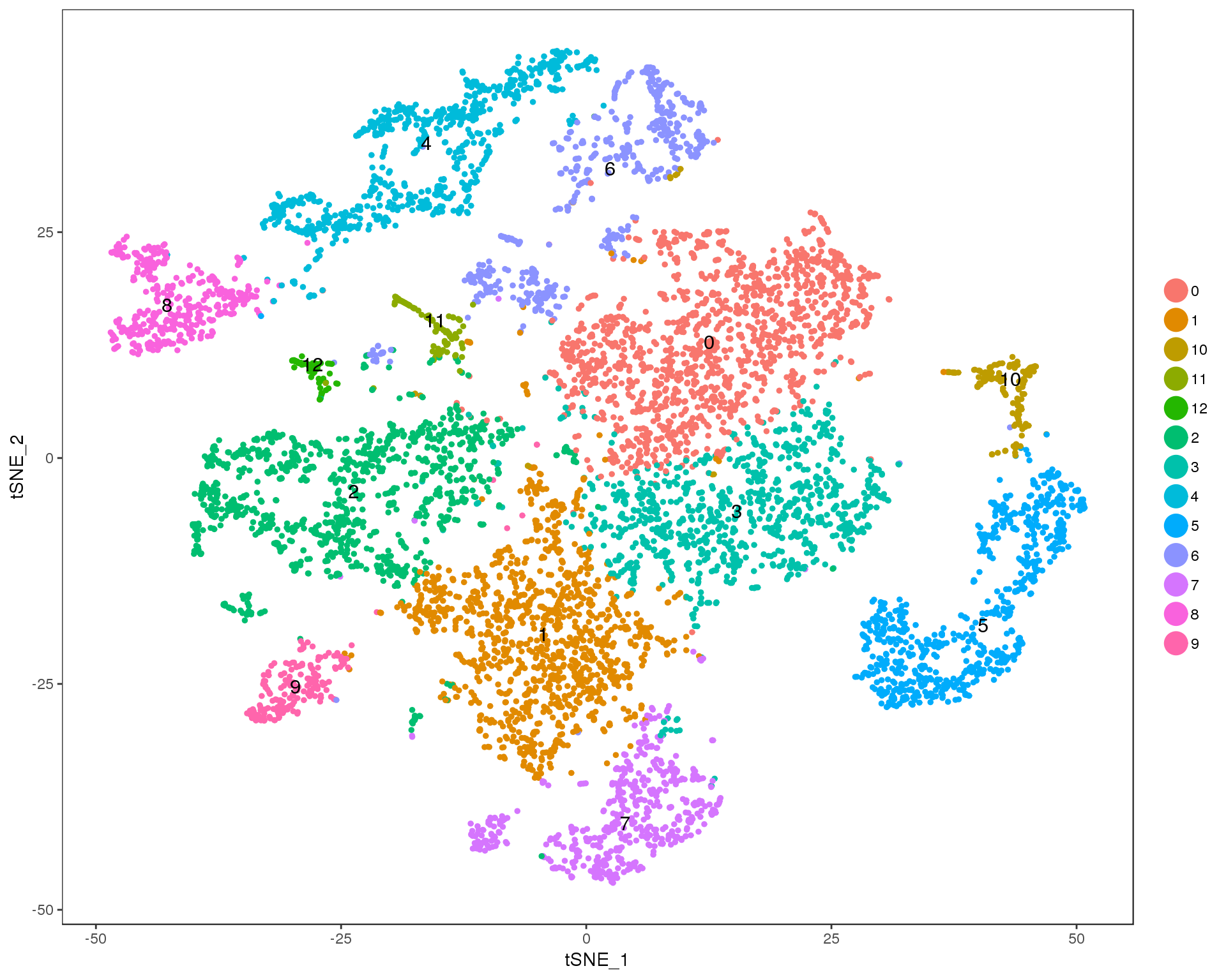
Res 0.5
TSNEPlot(seurat, group.by = 'res.0.5', do.label = TRUE)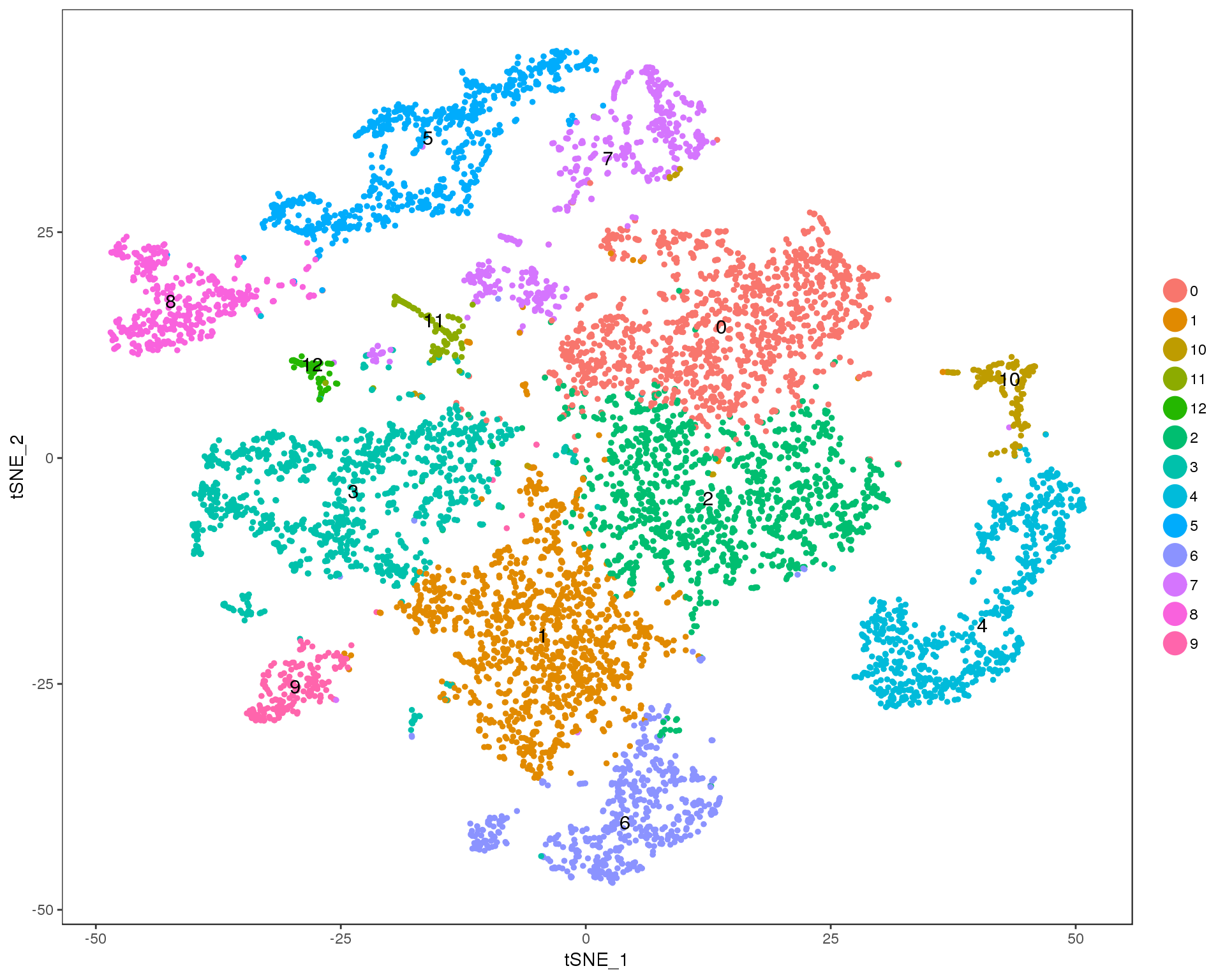
Res 0.6
TSNEPlot(seurat, group.by = 'res.0.6', do.label = TRUE)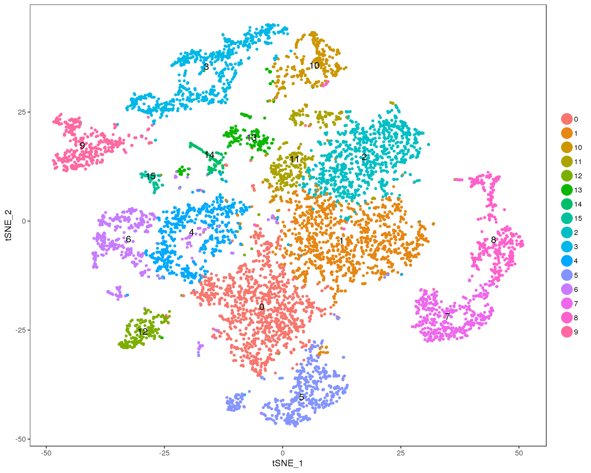
Res 0.7
TSNEPlot(seurat, group.by = 'res.0.7', do.label = TRUE)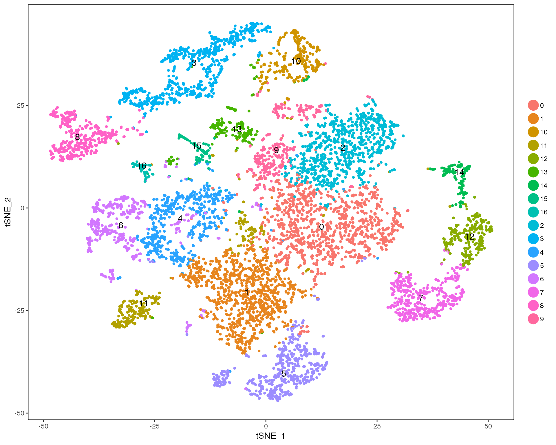
Res 0.8
TSNEPlot(seurat, group.by = 'res.0.8', do.label = TRUE)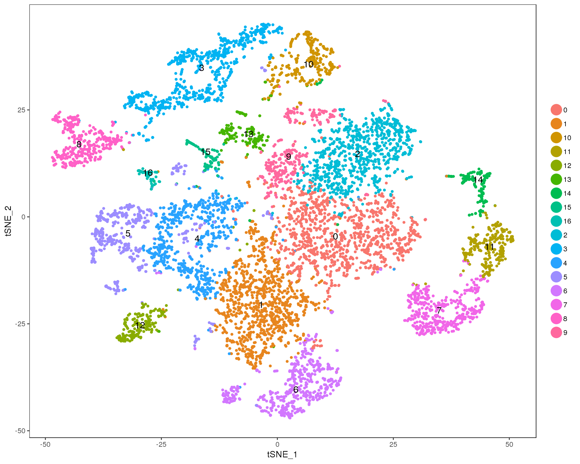
Res 0.9
TSNEPlot(seurat, group.by = 'res.0.9', do.label = TRUE)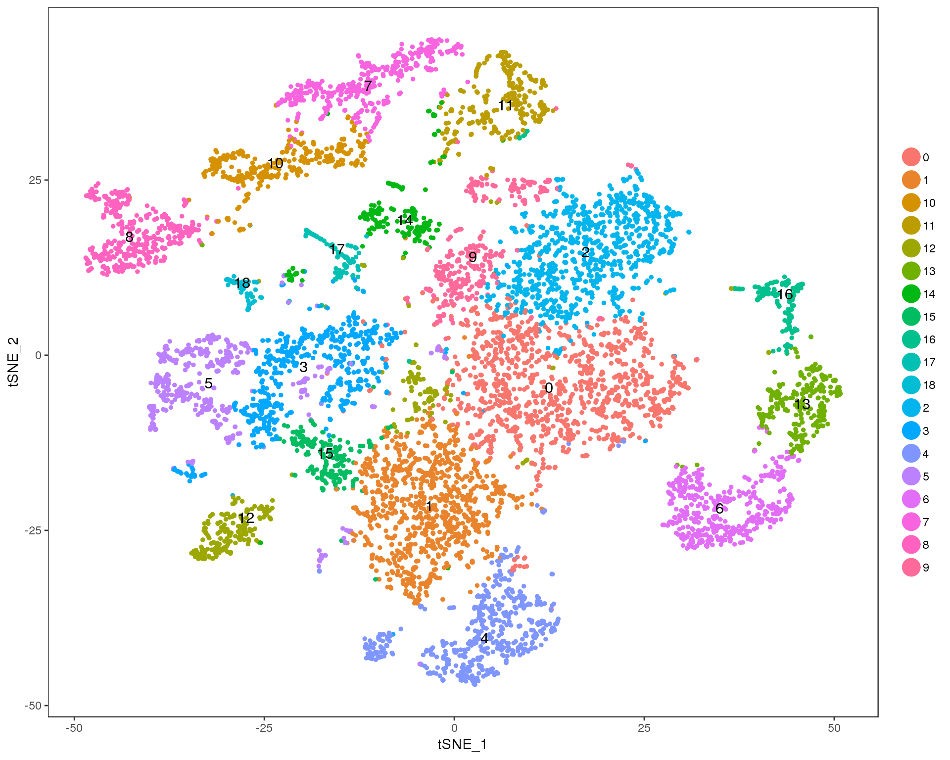
Clustering trees
Clustering trees show the relationship between clusterings at adjacent resolutions. Each cluster is represented as a node in a graph and the edges show the overlap between clusters.
Standard
Coloured by clustering resolution.
clustree(seurat)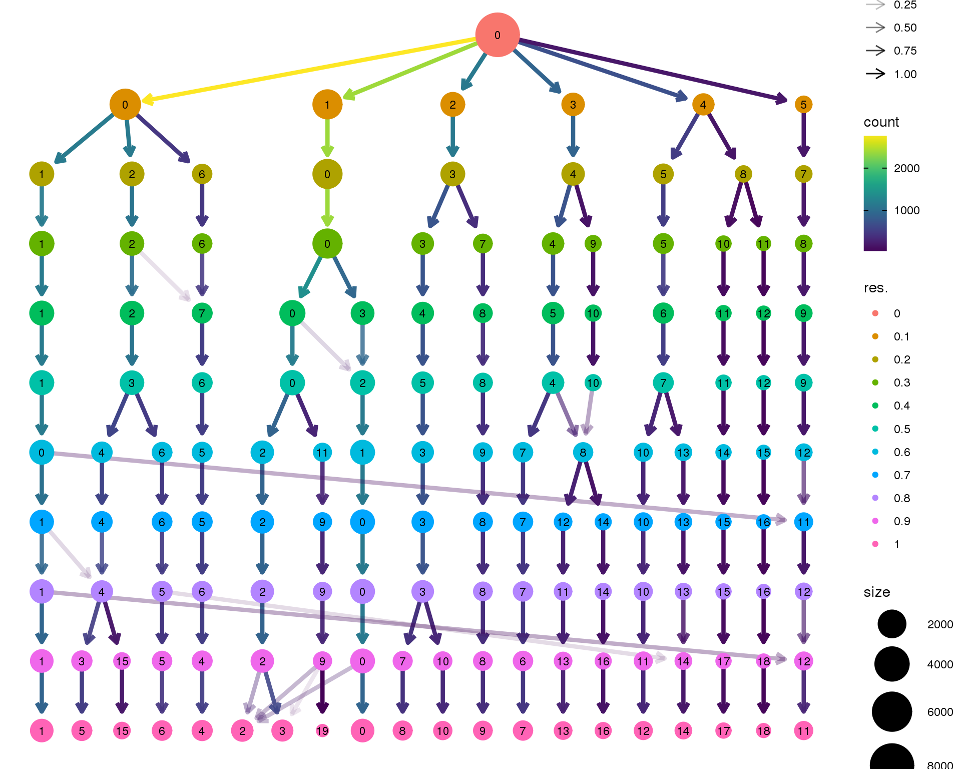
Stability
Coloured by the SC3 stability metric.
clustree(seurat, node_colour = "sc3_stability")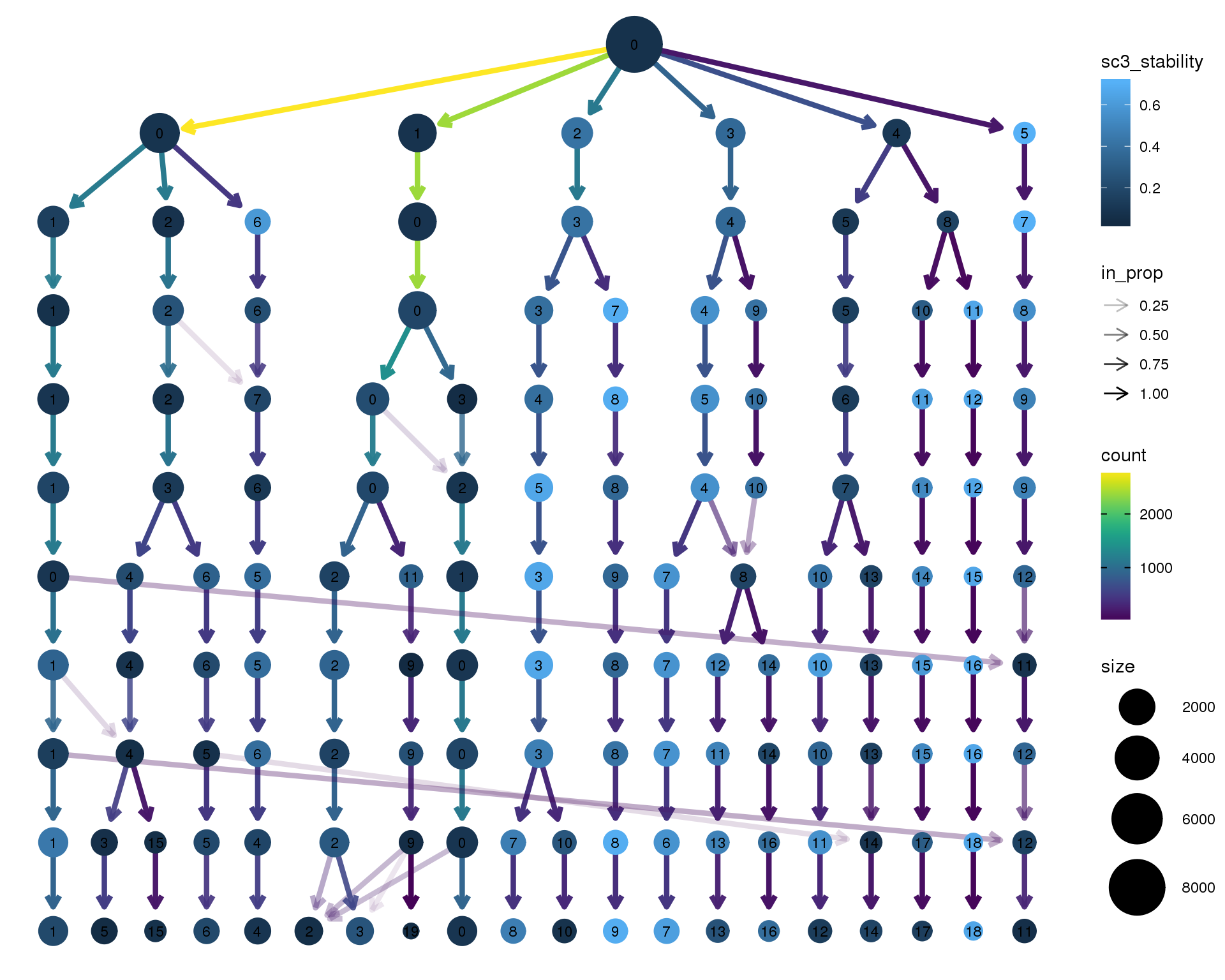
Genes
Coloured by the expression of known marker genes.
known_genes <- c(
    # Stroma
    "TAGLN", "ACTA2", "MAB21L2", "DLK1", "GATA3", "COL2A1", "COL9A3",
    # Podocyte
    "PODXL", "NPHS2", "TCF21",
    # Cell cycle
    "HIST1H4C", "PCLAF", "CENPF", "HMGB2",
    # Endothelium
    "CLDN5", "PECAM1", "KDR", "CALM1",
    # Neural
    "TTYH1", "SOX2", "HES6", "STMN2",
    # Epithelium
    "PAX2", "PAX8", "KRT19",
    # Muscle
    "MYOG", "MYOD1"
)

is_present <- known_genes %in% rownames(seurat@data)
The following genes aren’t present in this dataset and will be skipped:
src_list <- lapply(known_genes[is_present], function(gene) {
    src <- c("#### {{gene}} {.unnumbered}",
             "```{r clustree-{{gene}}}",
             "clustree(seurat, node_colour = '{{gene}}',",
                      "node_colour_aggr = 'mean', exprs = 'scale.data') +",
             "scale_colour_viridis_c(option = 'plasma', begin = 0.3)",
             "```",
             "")
    knit_expand(text = src)
})

out <- knit_child(text = unlist(src_list), options = list(cache = FALSE))
TAGLN
clustree(seurat, node_colour = 'TAGLN',
node_colour_aggr = 'mean', exprs = 'scale.data') +
scale_colour_viridis_c(option = 'plasma', begin = 0.3)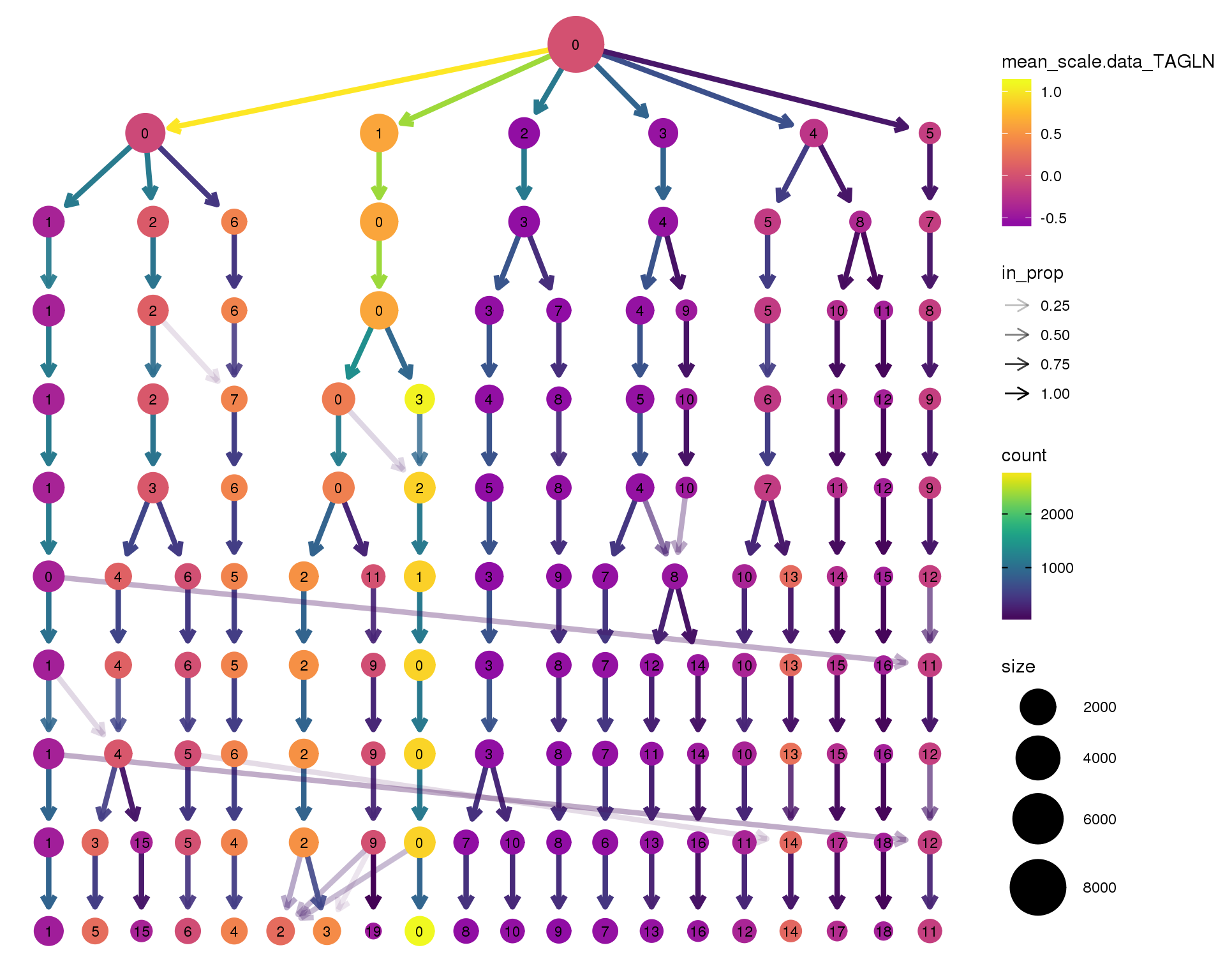
ACTA2
clustree(seurat, node_colour = 'ACTA2',
node_colour_aggr = 'mean', exprs = 'scale.data') +
scale_colour_viridis_c(option = 'plasma', begin = 0.3)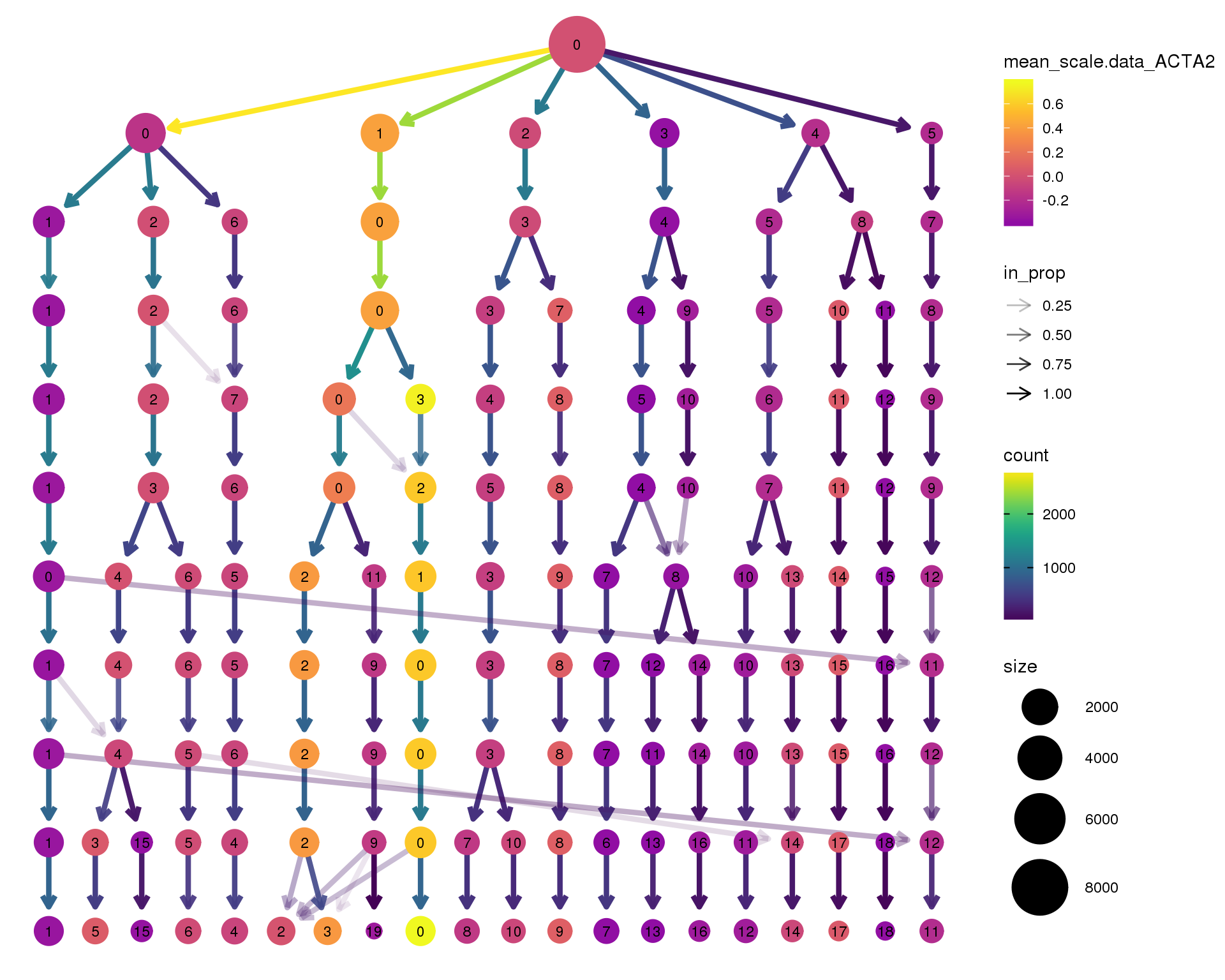
MAB21L2
clustree(seurat, node_colour = 'MAB21L2',
node_colour_aggr = 'mean', exprs = 'scale.data') +
scale_colour_viridis_c(option = 'plasma', begin = 0.3)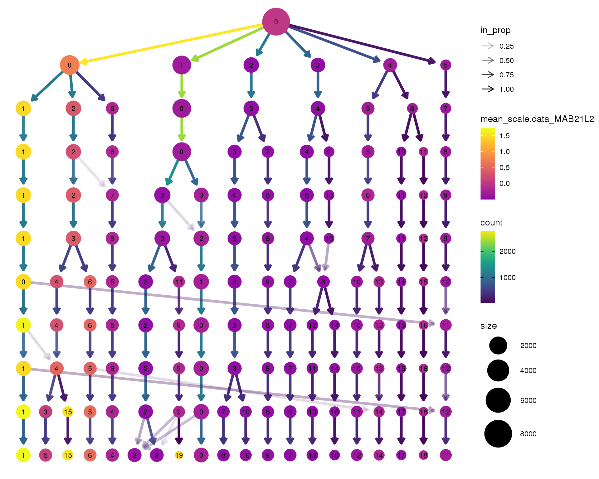
DLK1
clustree(seurat, node_colour = 'DLK1',
node_colour_aggr = 'mean', exprs = 'scale.data') +
scale_colour_viridis_c(option = 'plasma', begin = 0.3)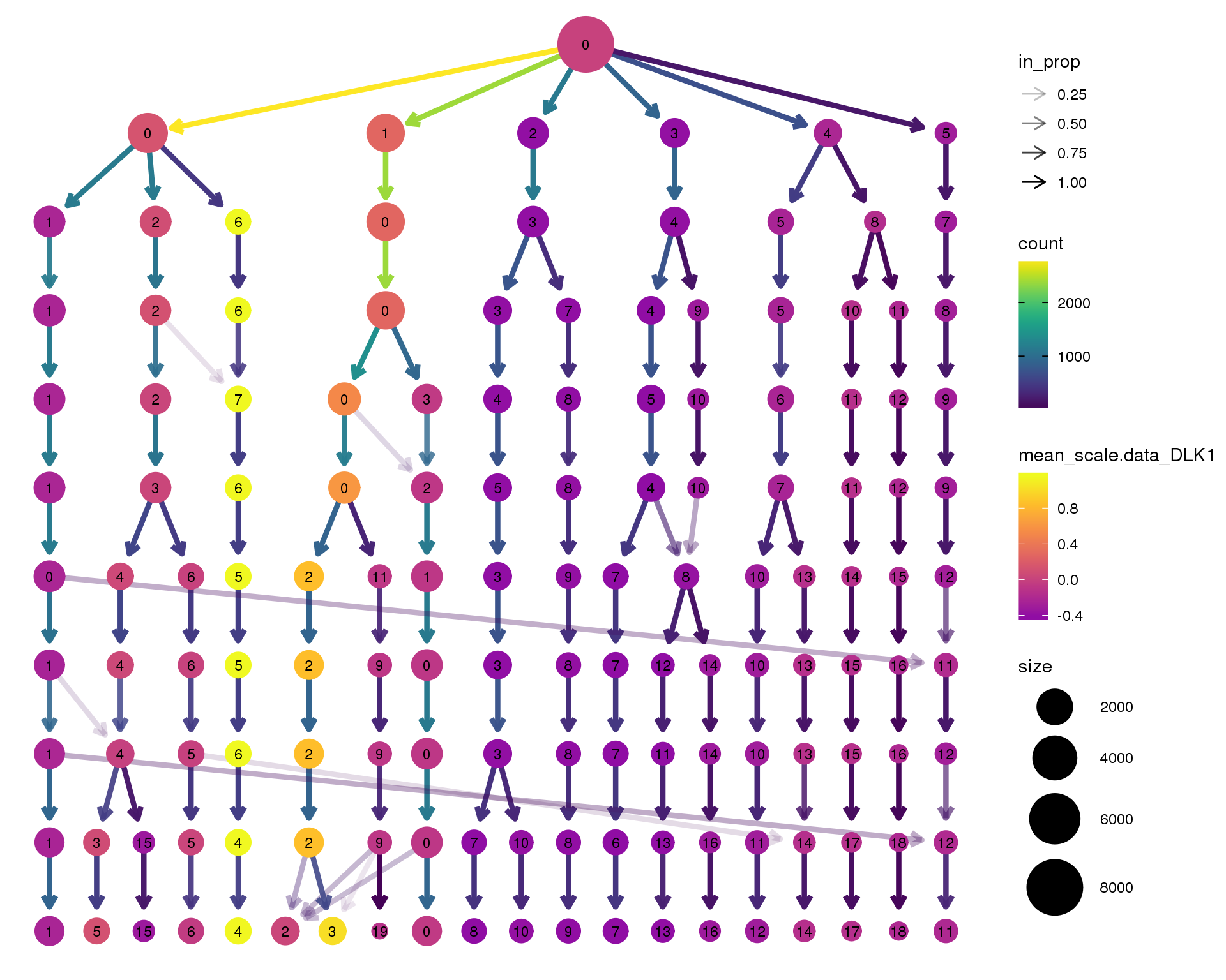
GATA3
clustree(seurat, node_colour = 'GATA3',
node_colour_aggr = 'mean', exprs = 'scale.data') +
scale_colour_viridis_c(option = 'plasma', begin = 0.3)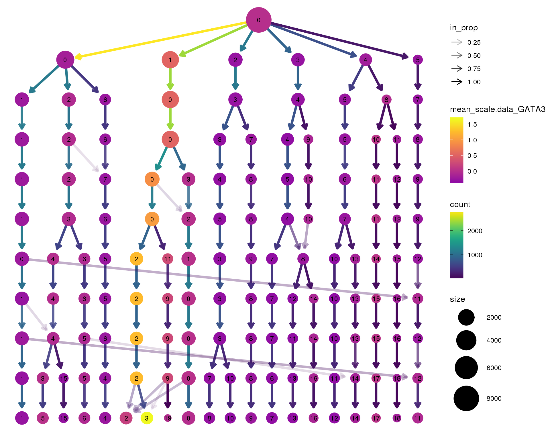
COL2A1
clustree(seurat, node_colour = 'COL2A1',
node_colour_aggr = 'mean', exprs = 'scale.data') +
scale_colour_viridis_c(option = 'plasma', begin = 0.3)
COL9A3
clustree(seurat, node_colour = 'COL9A3',
node_colour_aggr = 'mean', exprs = 'scale.data') +
scale_colour_viridis_c(option = 'plasma', begin = 0.3)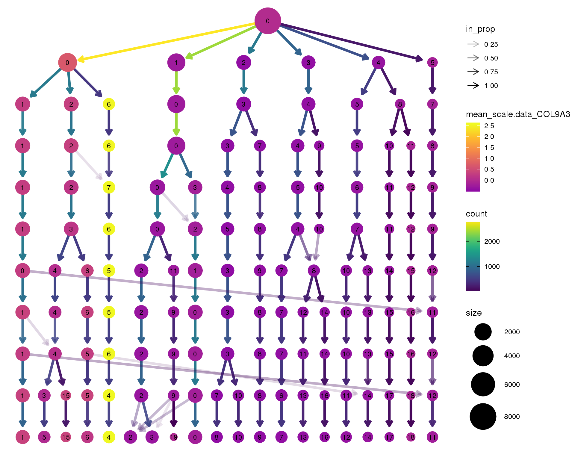
PODXL
clustree(seurat, node_colour = 'PODXL',
node_colour_aggr = 'mean', exprs = 'scale.data') +
scale_colour_viridis_c(option = 'plasma', begin = 0.3)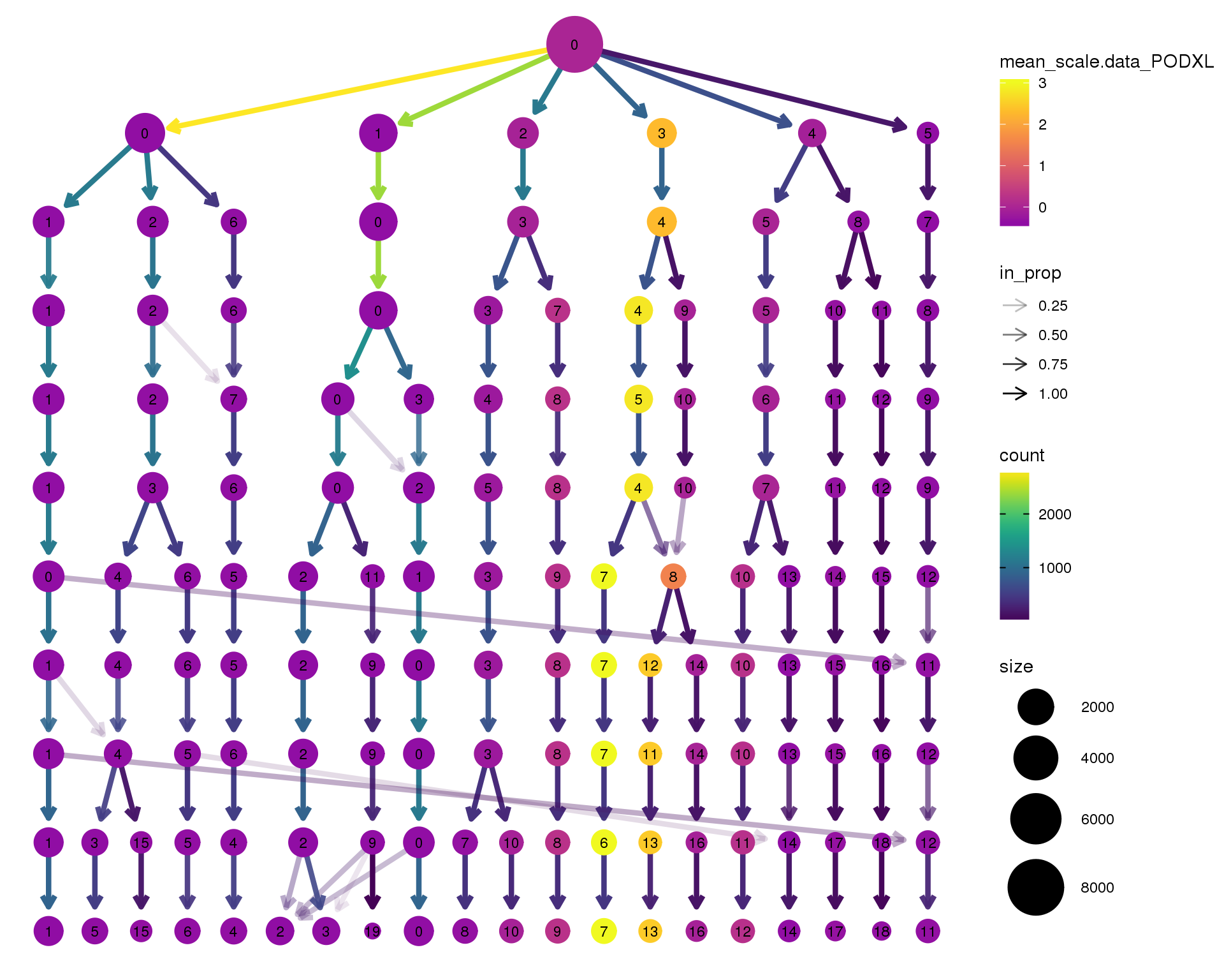
NPHS2
clustree(seurat, node_colour = 'NPHS2',
node_colour_aggr = 'mean', exprs = 'scale.data') +
scale_colour_viridis_c(option = 'plasma', begin = 0.3)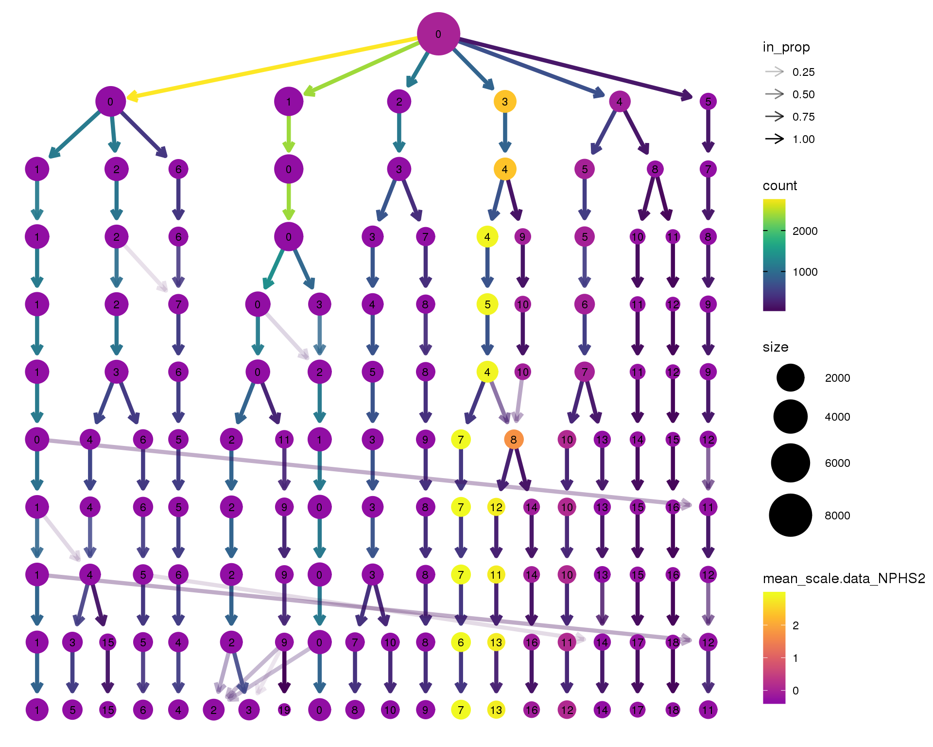
TCF21
clustree(seurat, node_colour = 'TCF21',
node_colour_aggr = 'mean', exprs = 'scale.data') +
scale_colour_viridis_c(option = 'plasma', begin = 0.3)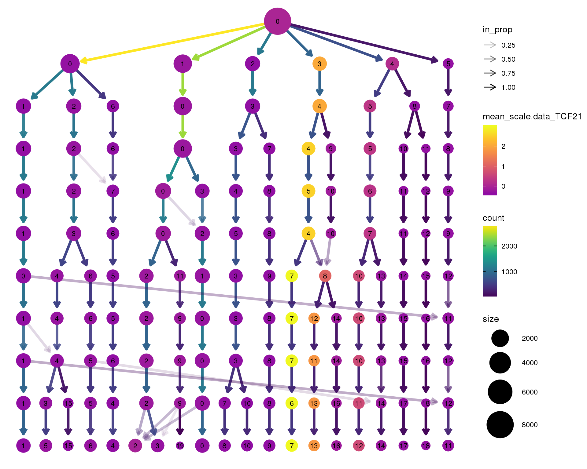
HIST1H4C
clustree(seurat, node_colour = 'HIST1H4C',
node_colour_aggr = 'mean', exprs = 'scale.data') +
scale_colour_viridis_c(option = 'plasma', begin = 0.3)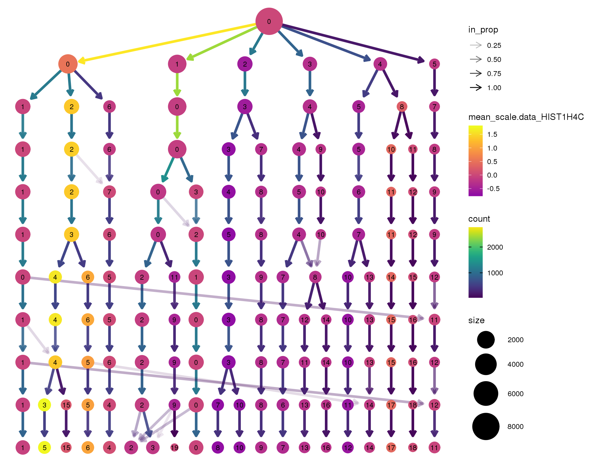
PCLAF
clustree(seurat, node_colour = 'PCLAF',
node_colour_aggr = 'mean', exprs = 'scale.data') +
scale_colour_viridis_c(option = 'plasma', begin = 0.3)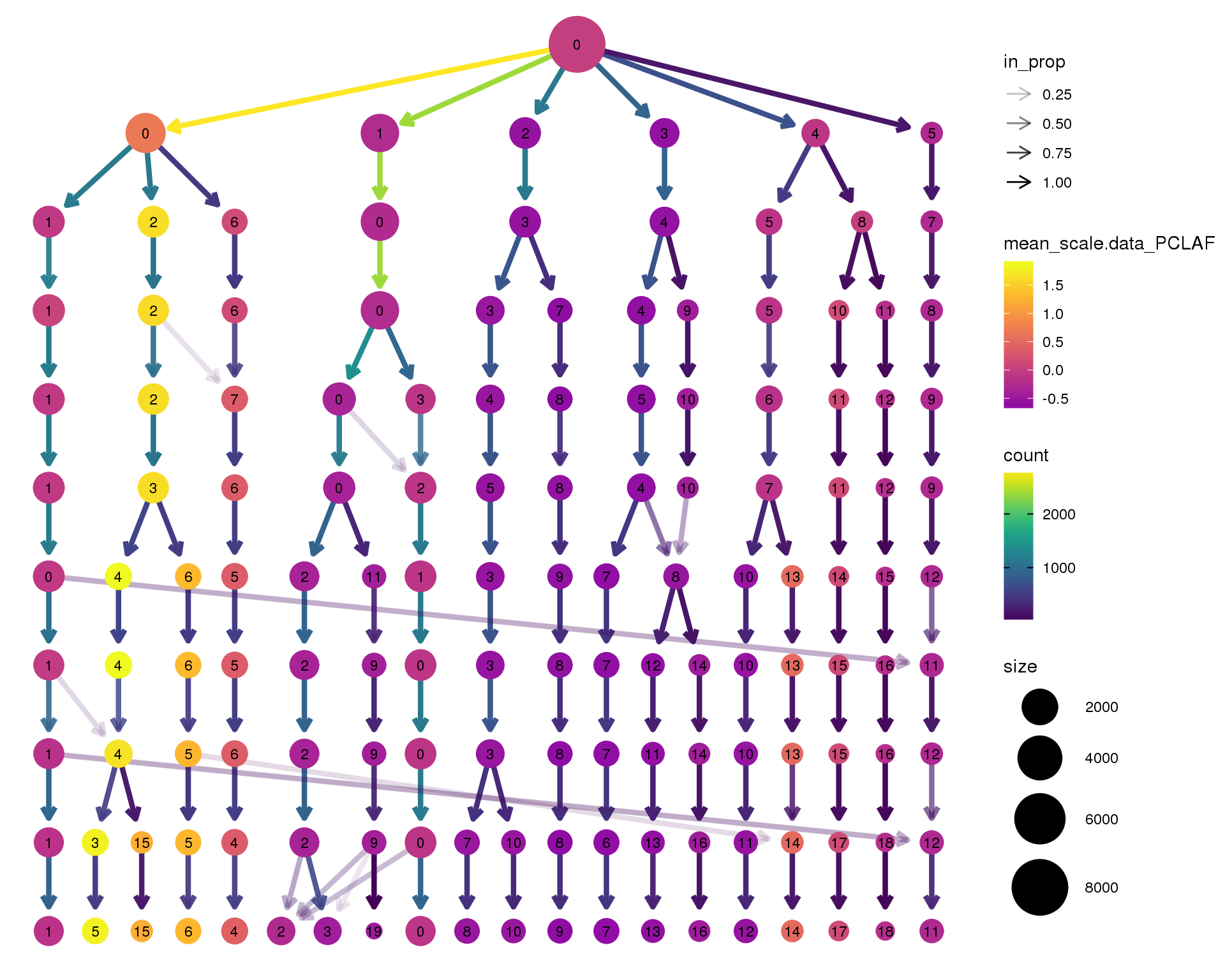
CENPF
clustree(seurat, node_colour = 'CENPF',
node_colour_aggr = 'mean', exprs = 'scale.data') +
scale_colour_viridis_c(option = 'plasma', begin = 0.3)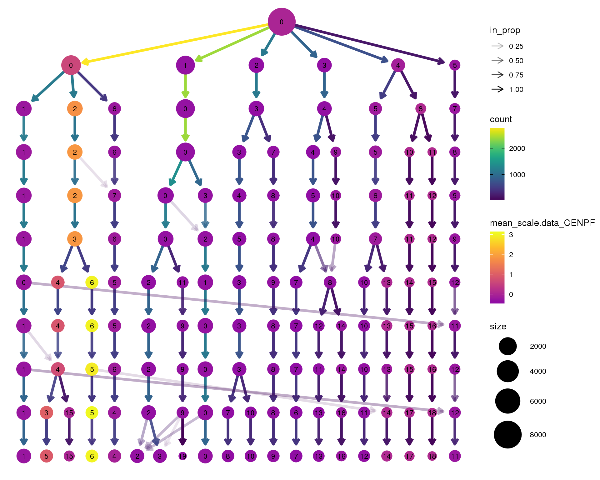
HMGB2
clustree(seurat, node_colour = 'HMGB2',
node_colour_aggr = 'mean', exprs = 'scale.data') +
scale_colour_viridis_c(option = 'plasma', begin = 0.3)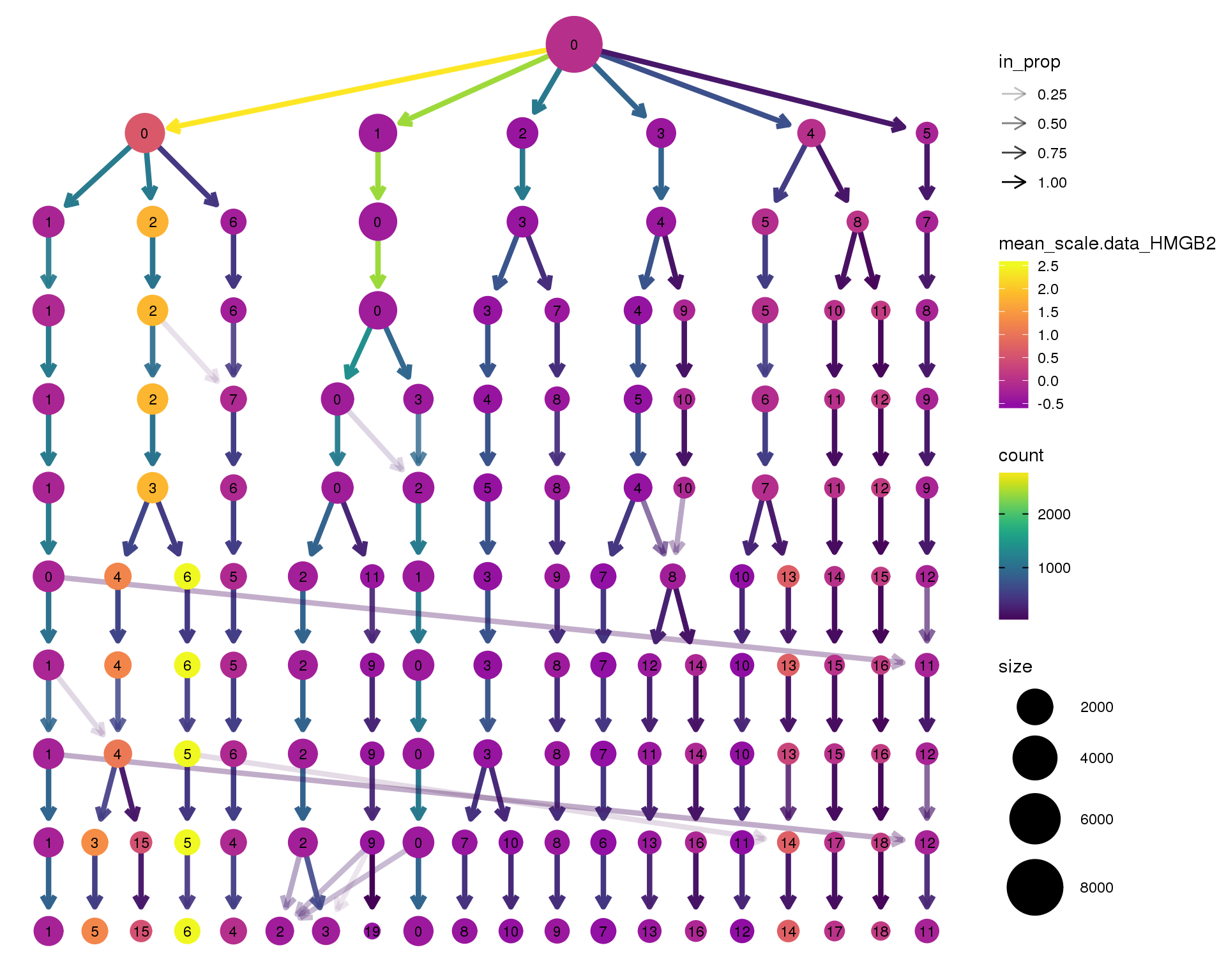
CLDN5
clustree(seurat, node_colour = 'CLDN5',
node_colour_aggr = 'mean', exprs = 'scale.data') +
scale_colour_viridis_c(option = 'plasma', begin = 0.3)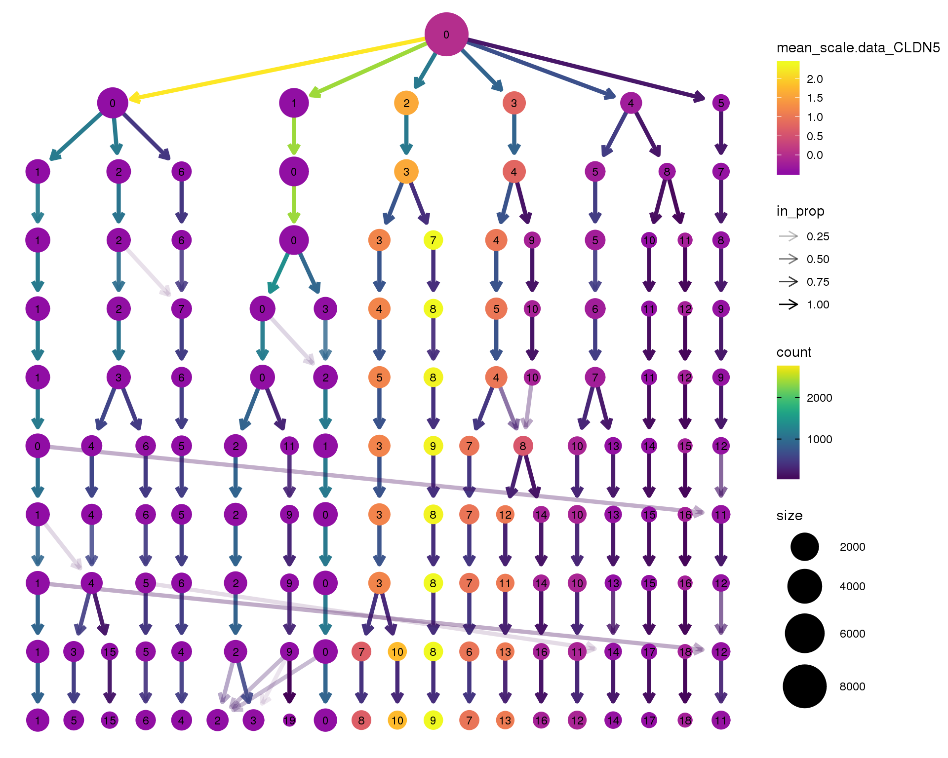
PECAM1
clustree(seurat, node_colour = 'PECAM1',
node_colour_aggr = 'mean', exprs = 'scale.data') +
scale_colour_viridis_c(option = 'plasma', begin = 0.3)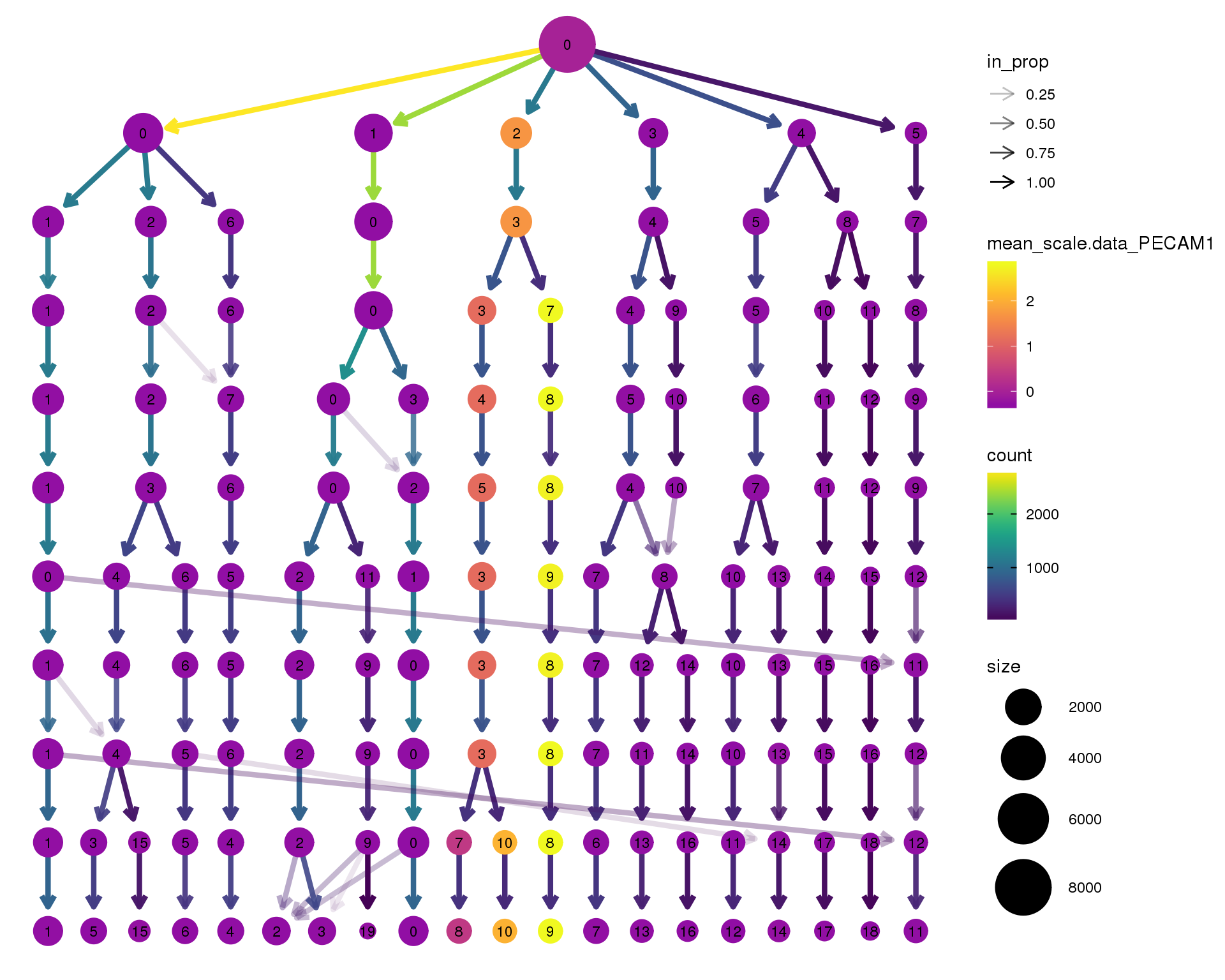
KDR
clustree(seurat, node_colour = 'KDR',
node_colour_aggr = 'mean', exprs = 'scale.data') +
scale_colour_viridis_c(option = 'plasma', begin = 0.3)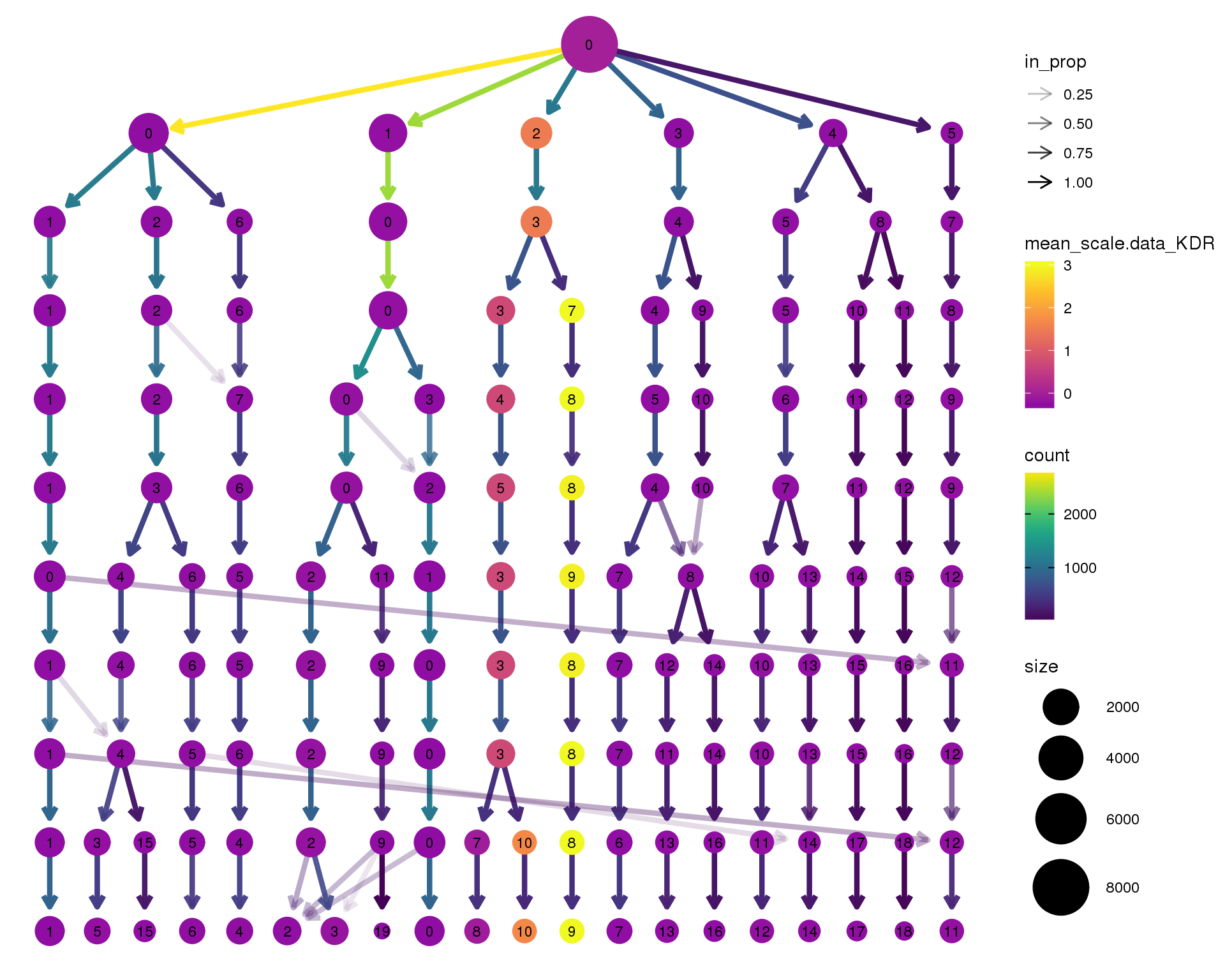
CALM1
clustree(seurat, node_colour = 'CALM1',
node_colour_aggr = 'mean', exprs = 'scale.data') +
scale_colour_viridis_c(option = 'plasma', begin = 0.3)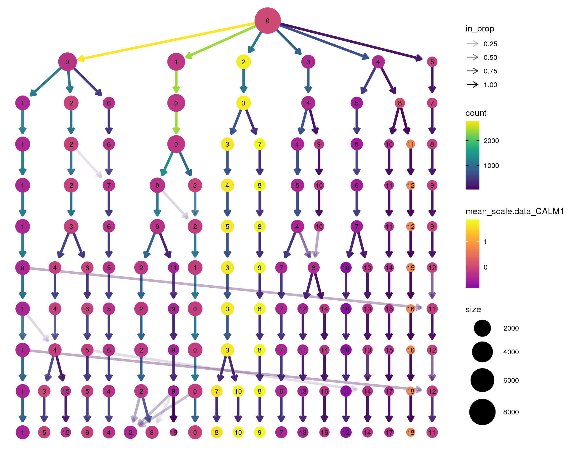
TTYH1
clustree(seurat, node_colour = 'TTYH1',
node_colour_aggr = 'mean', exprs = 'scale.data') +
scale_colour_viridis_c(option = 'plasma', begin = 0.3)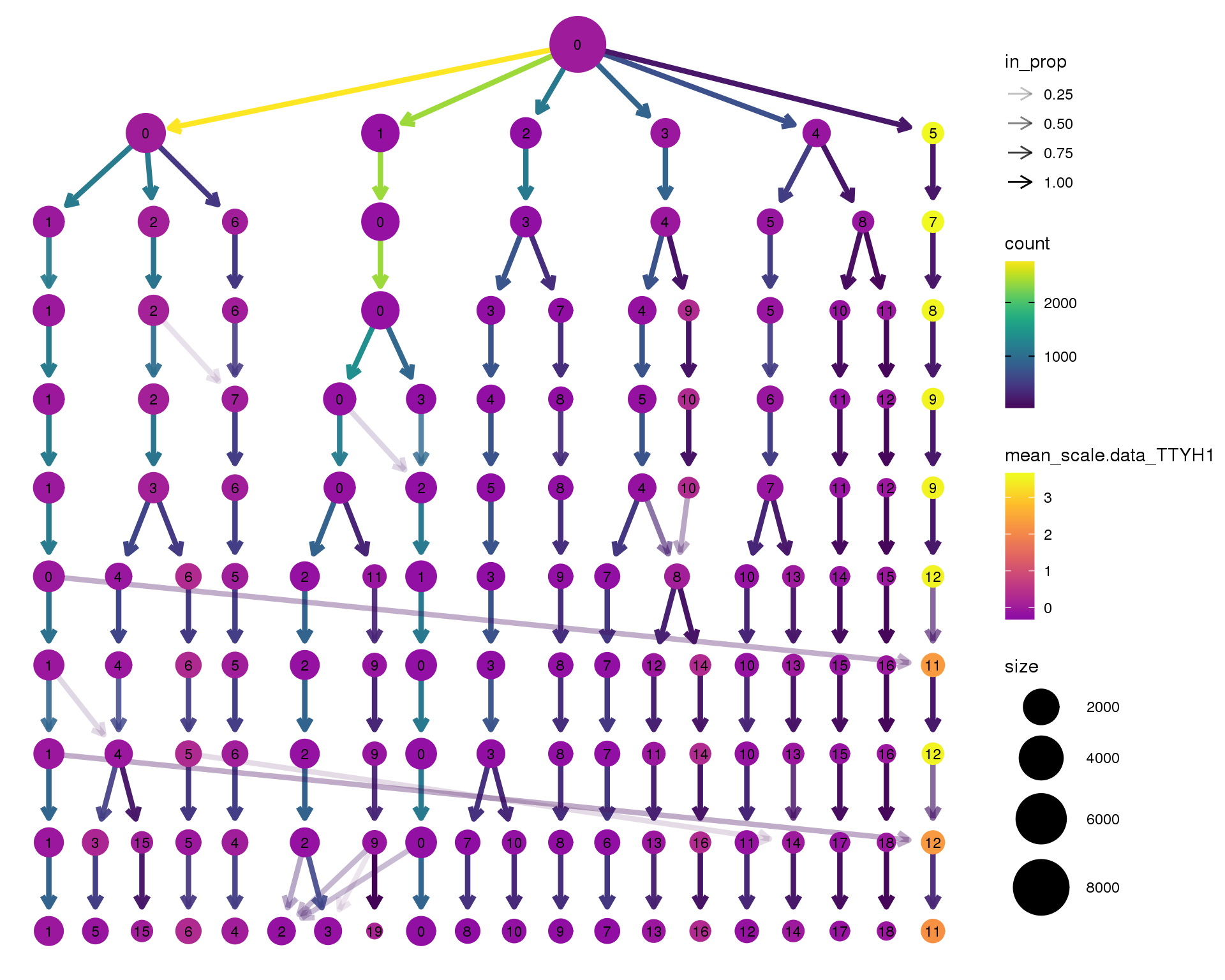
SOX2
clustree(seurat, node_colour = 'SOX2',
node_colour_aggr = 'mean', exprs = 'scale.data') +
scale_colour_viridis_c(option = 'plasma', begin = 0.3)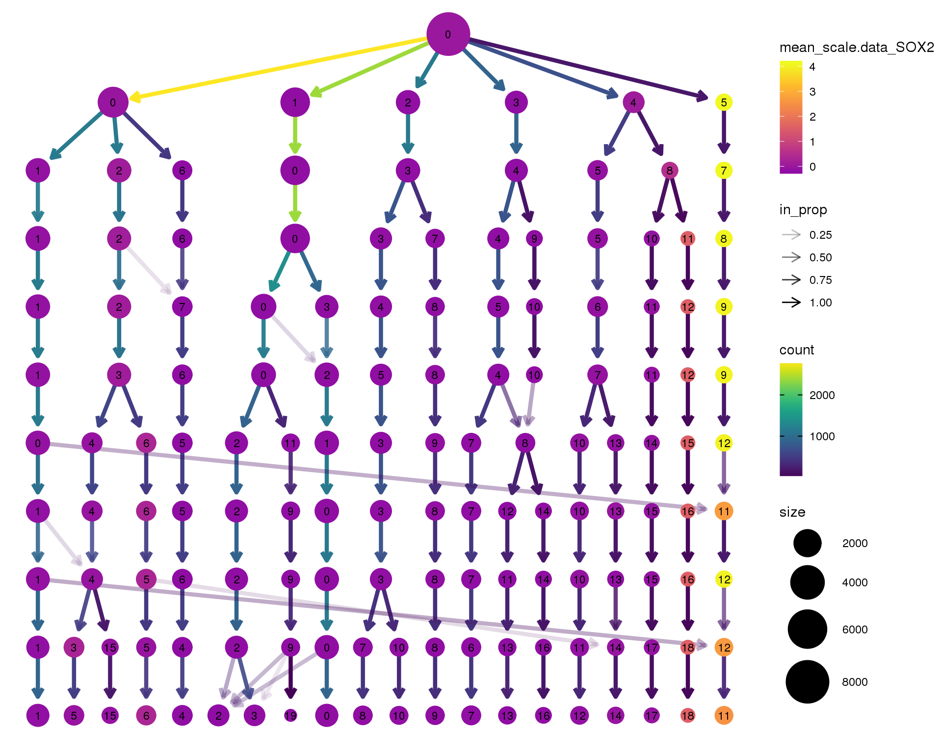
HES6
clustree(seurat, node_colour = 'HES6',
node_colour_aggr = 'mean', exprs = 'scale.data') +
scale_colour_viridis_c(option = 'plasma', begin = 0.3)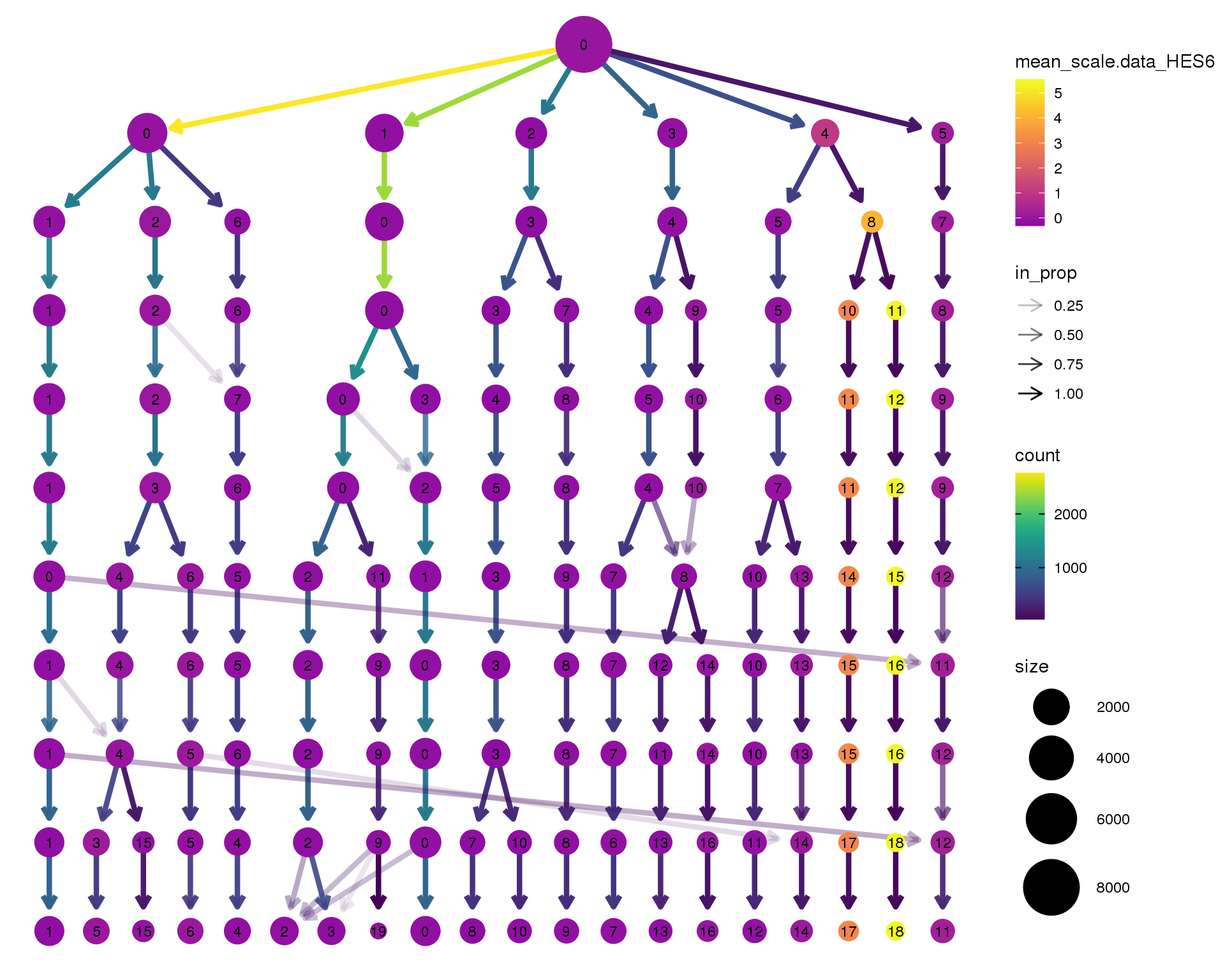
STMN2
clustree(seurat, node_colour = 'STMN2',
node_colour_aggr = 'mean', exprs = 'scale.data') +
scale_colour_viridis_c(option = 'plasma', begin = 0.3)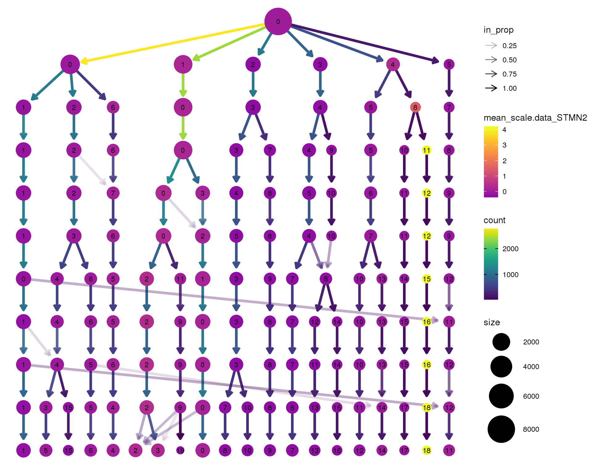
PAX2
clustree(seurat, node_colour = 'PAX2',
node_colour_aggr = 'mean', exprs = 'scale.data') +
scale_colour_viridis_c(option = 'plasma', begin = 0.3)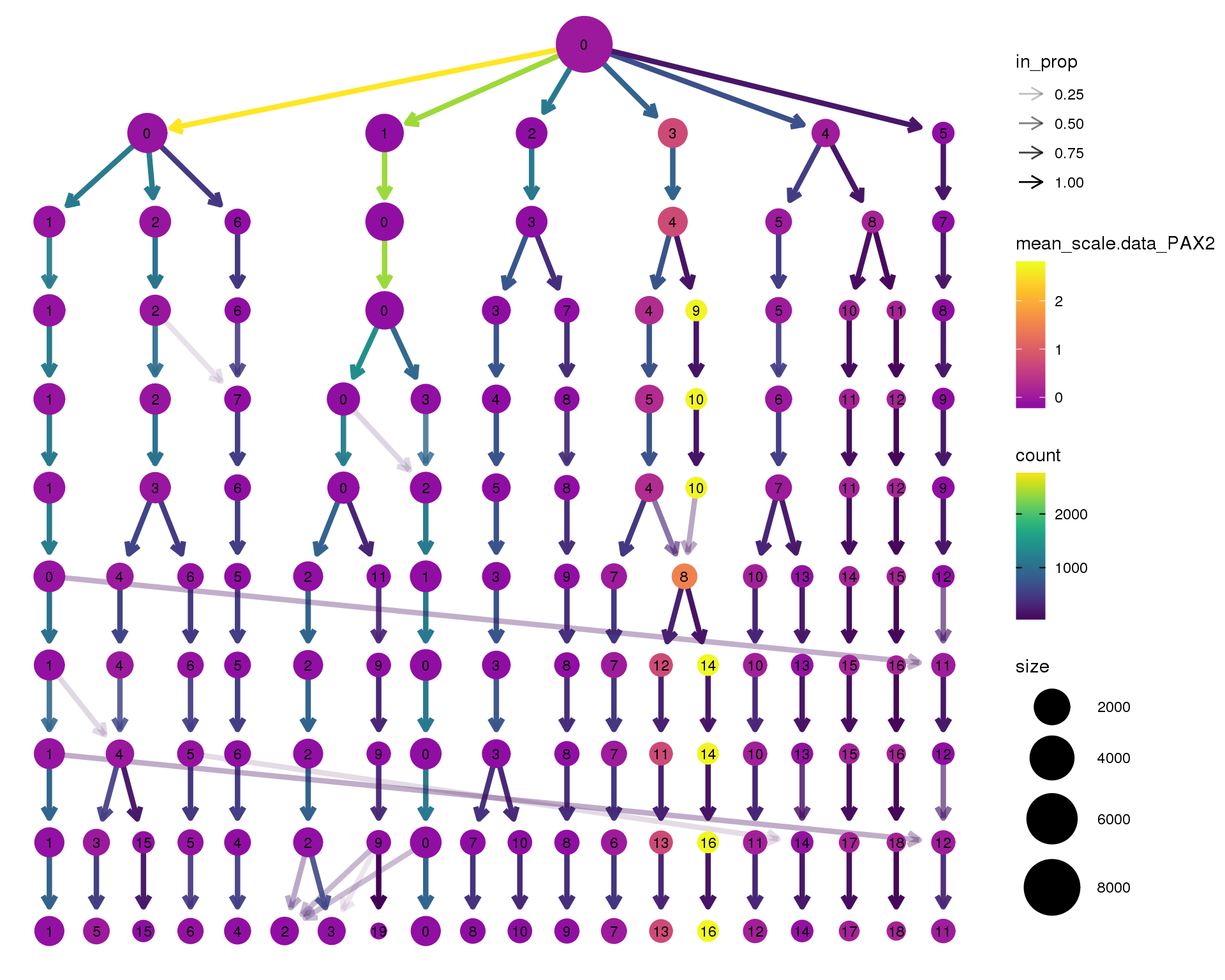
PAX8
clustree(seurat, node_colour = 'PAX8',
node_colour_aggr = 'mean', exprs = 'scale.data') +
scale_colour_viridis_c(option = 'plasma', begin = 0.3)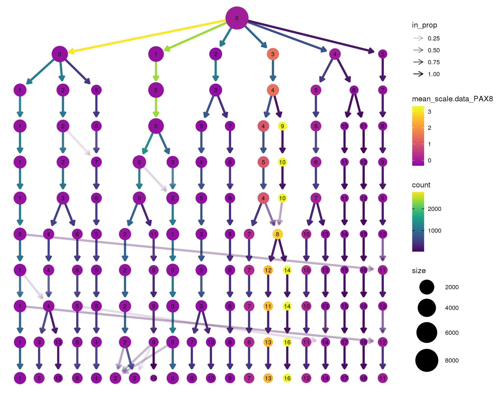
KRT19
clustree(seurat, node_colour = 'KRT19',
node_colour_aggr = 'mean', exprs = 'scale.data') +
scale_colour_viridis_c(option = 'plasma', begin = 0.3)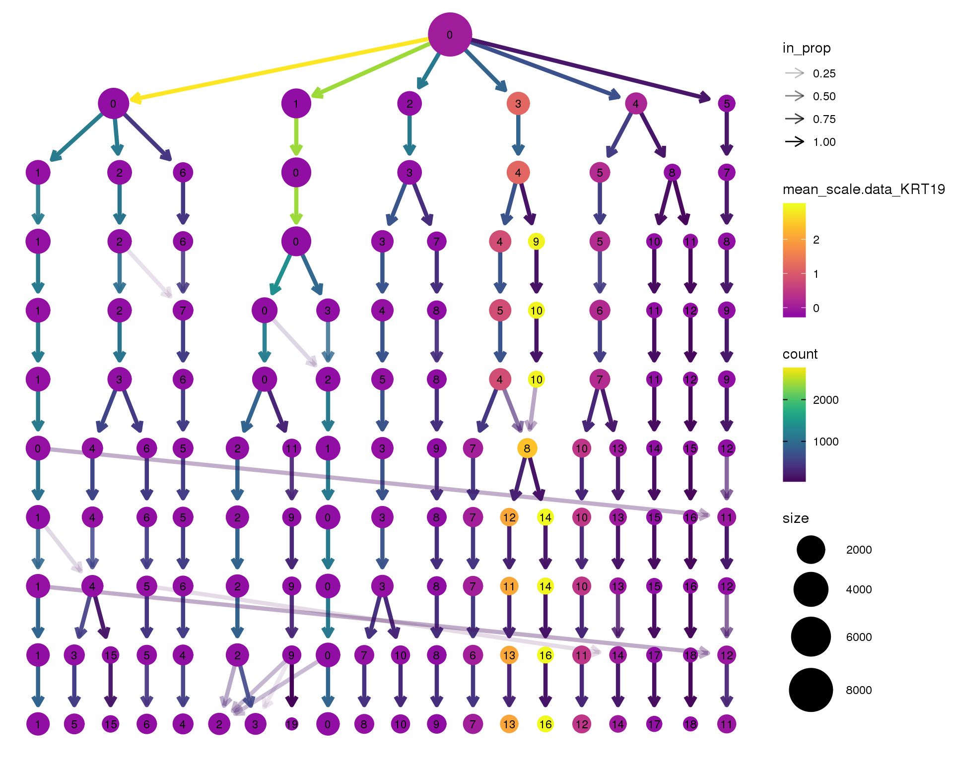
MYOG
clustree(seurat, node_colour = 'MYOG',
node_colour_aggr = 'mean', exprs = 'scale.data') +
scale_colour_viridis_c(option = 'plasma', begin = 0.3)
MYOD1
clustree(seurat, node_colour = 'MYOD1',
node_colour_aggr = 'mean', exprs = 'scale.data') +
scale_colour_viridis_c(option = 'plasma', begin = 0.3)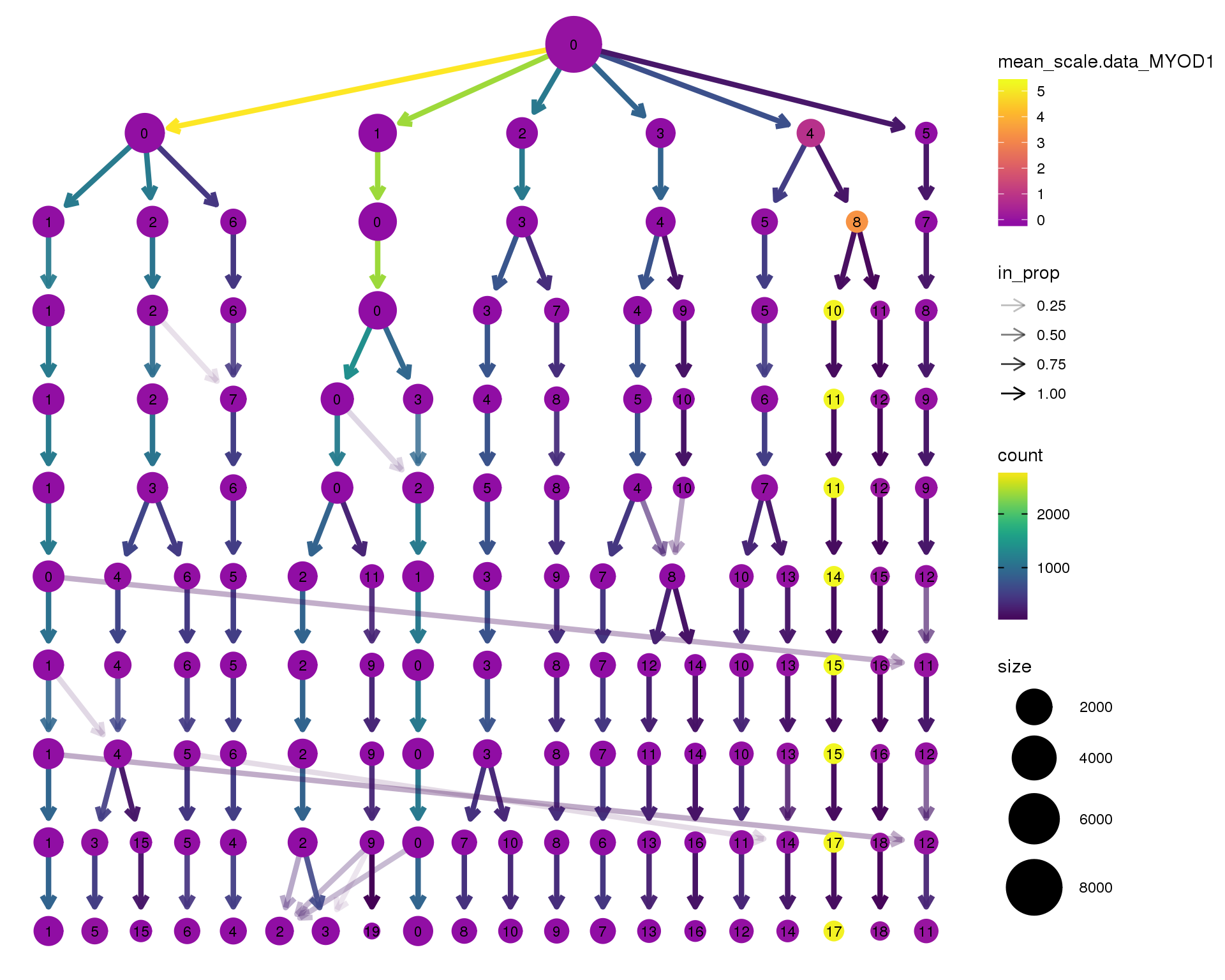
Selection
res <- 0.4
seurat <- SetIdent(seurat, ident.use = seurat@meta.data[, paste0("res.", res)])
n_clusts <- length(unique(seurat@ident))

colData(sce)$Cluster <- seurat@ident
reducedDim(sce, "SeuratPCA") <- seurat@dr$pca@cell.embeddings
reducedDim(sce, "SeuratGenesPCA") <- seurat@dr$pca_seurat@cell.embeddings
reducedDim(sce, "M3DropPCA") <- seurat@dr$pca_m3drop@cell.embeddings
reducedDim(sce, "SeuratTSNE") <- seurat@dr$tsne@cell.embeddings

umap <- reducedDim(sce, "UMAP")
sce <- runUMAP(sce, use_dimred = "SeuratPCA", n_dimred = n_pcs)
reducedDim(sce, "SeuratUMAP") <- reducedDim(sce, "UMAP")
reducedDim(sce, "UMAP") <- umap

cell_data <- as.data.frame(colData(sce))
Based on these plots we will use a resolution of 0.4 which gives us 13 clusters.
Validation
To validate the clusters we will repeat some of our quality control plots separated by cluster. At this stage we just want to check that none of the clusters are obviously the result of technical factors.
Cluster
Clusters assigned by Seurat.
Count
ggplot(cell_data, aes(x = Cluster, fill = Cluster)) +
    geom_bar() +
    theme_minimal()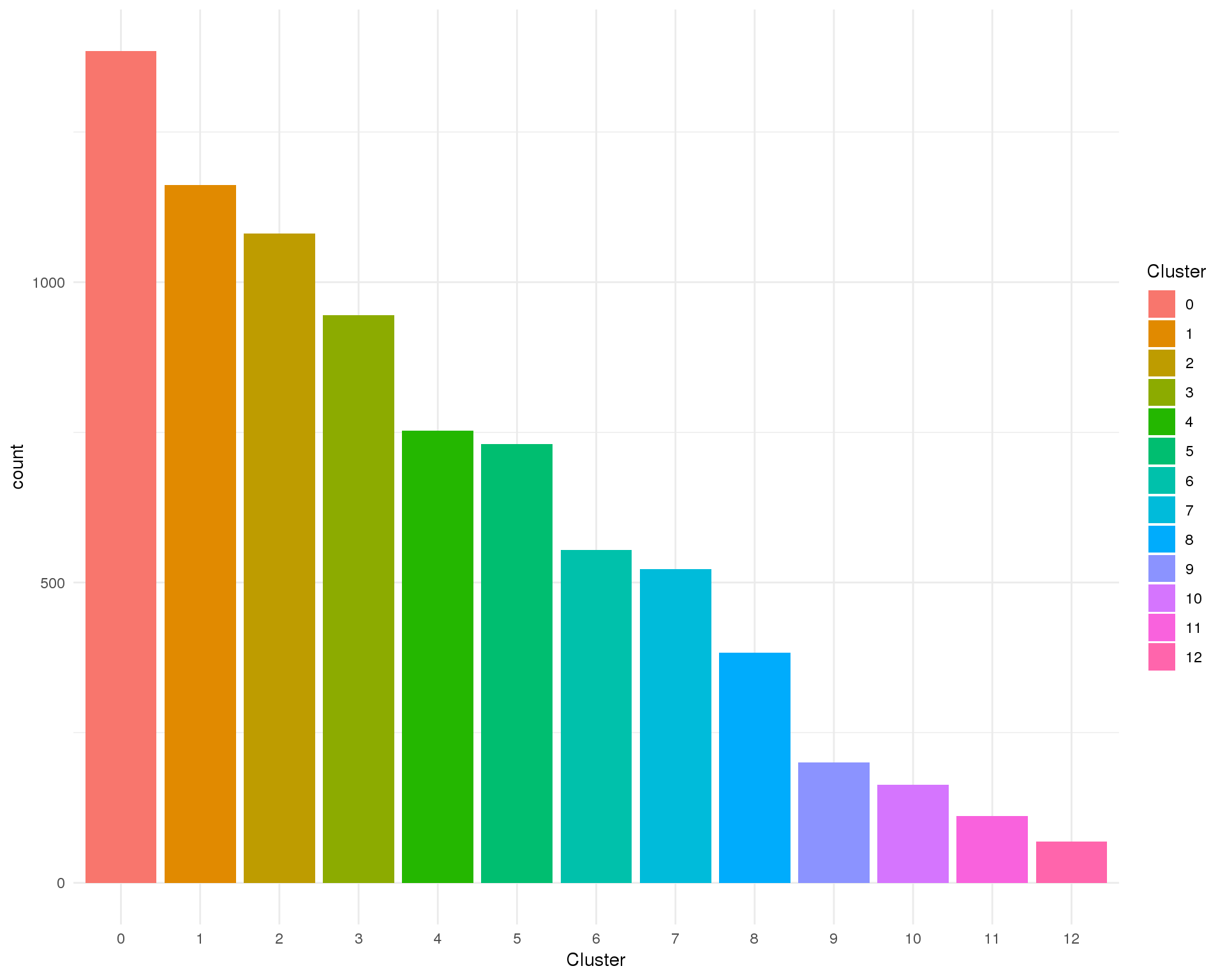
PCA
plotReducedDim(sce, "SeuratPCA", colour_by = "Cluster", add_ticks = FALSE,
               point_alpha = 1) +
    scale_fill_discrete() +
    theme_minimal()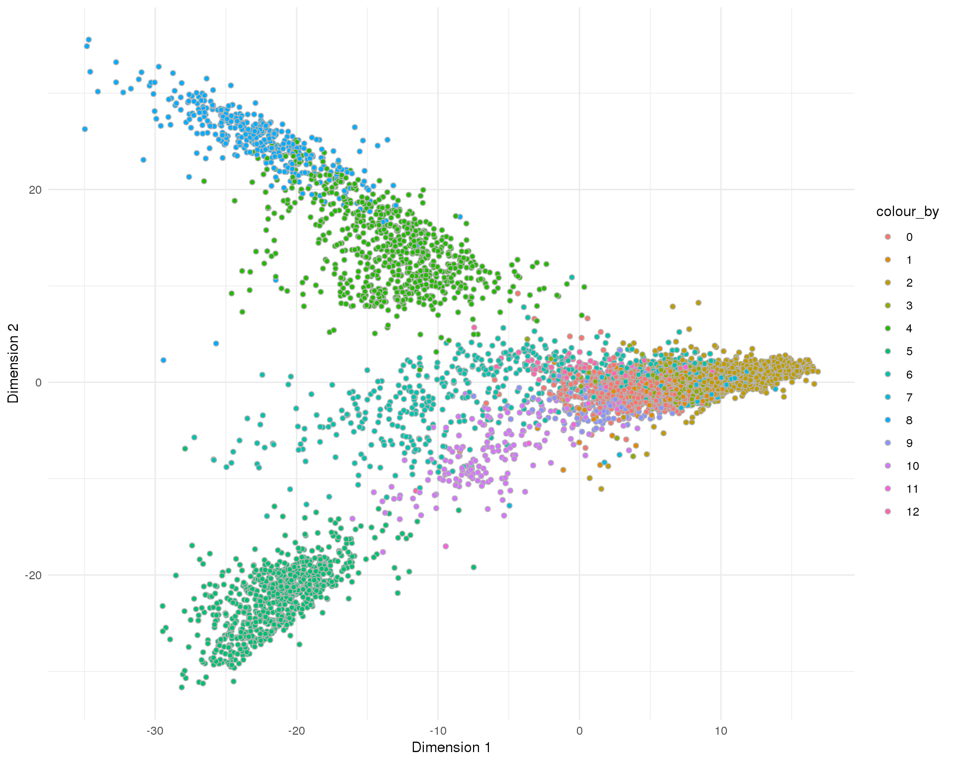
t-SNE
plotReducedDim(sce, "SeuratTSNE", colour_by = "Cluster", add_ticks = FALSE,
               point_alpha = 1) +
    scale_fill_discrete() +
    theme_minimal()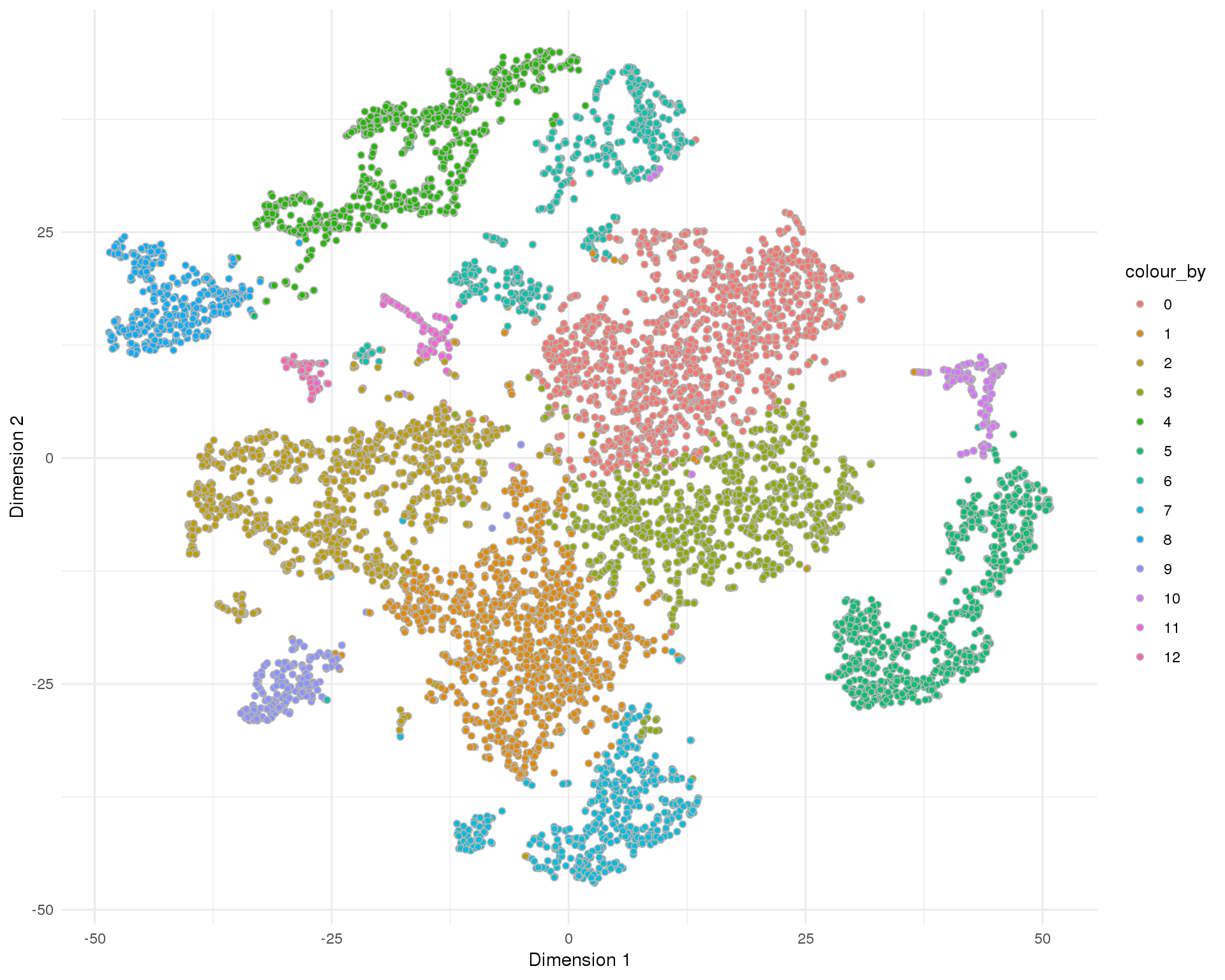
UMAP
plotReducedDim(sce, "SeuratUMAP", colour_by = "Cluster", add_ticks = FALSE,
               point_alpha = 1) +
    scale_fill_discrete() +
    theme_minimal()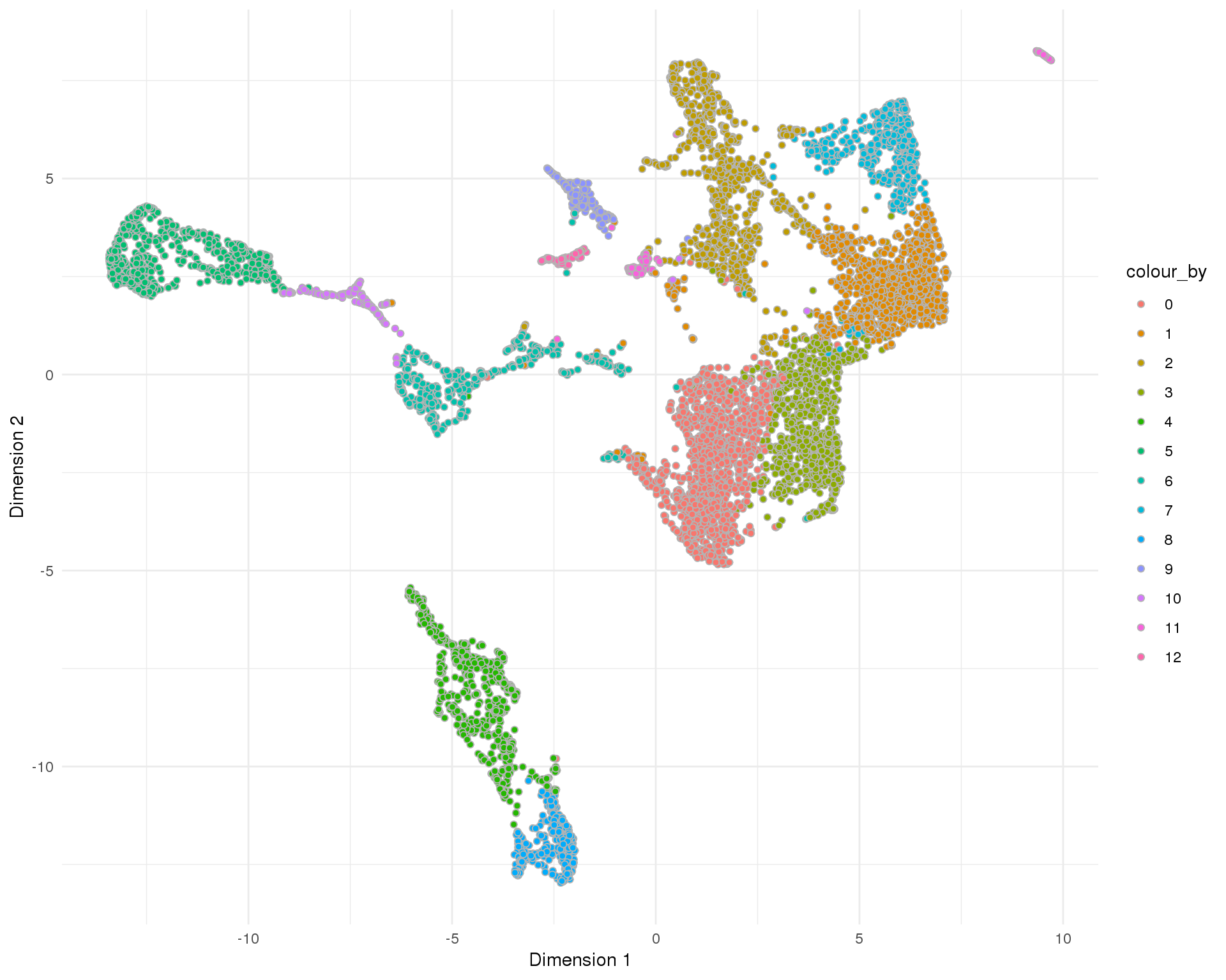
Sample
Biological sample.
Count
ggplot(cell_data, aes(x = Cluster, fill = Sample)) +
    geom_bar() +
    theme_minimal()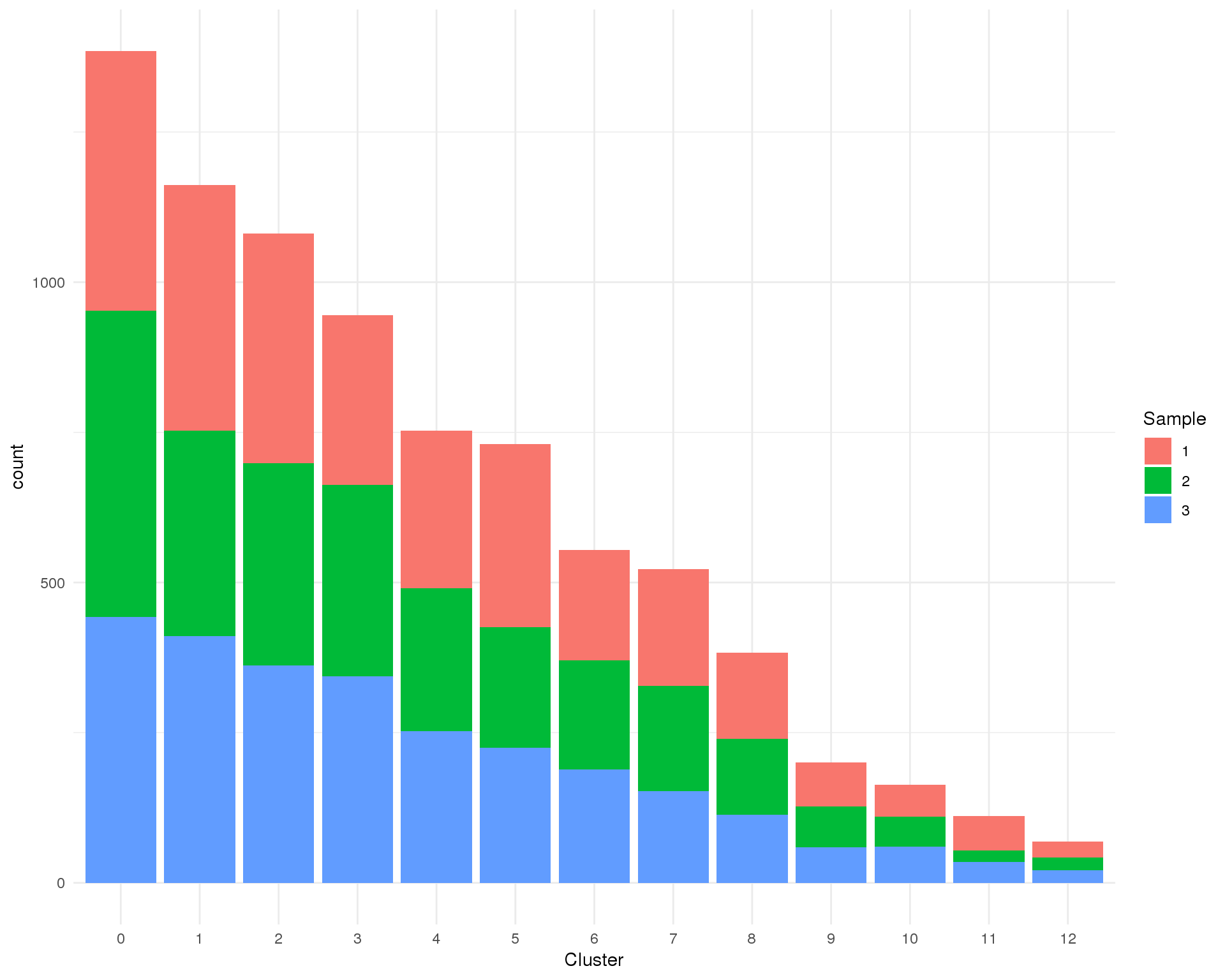
Proportion
plot_data <- cell_data %>%
    group_by(Cluster, Sample) %>%
    summarise(Count = n()) %>%
    mutate(Prop = Count / sum(Count))

ggplot(plot_data, aes(x = Cluster, y = Prop, fill = Sample)) +
    geom_col() +
    ylab("Proportion of cluster") +
    theme_minimal()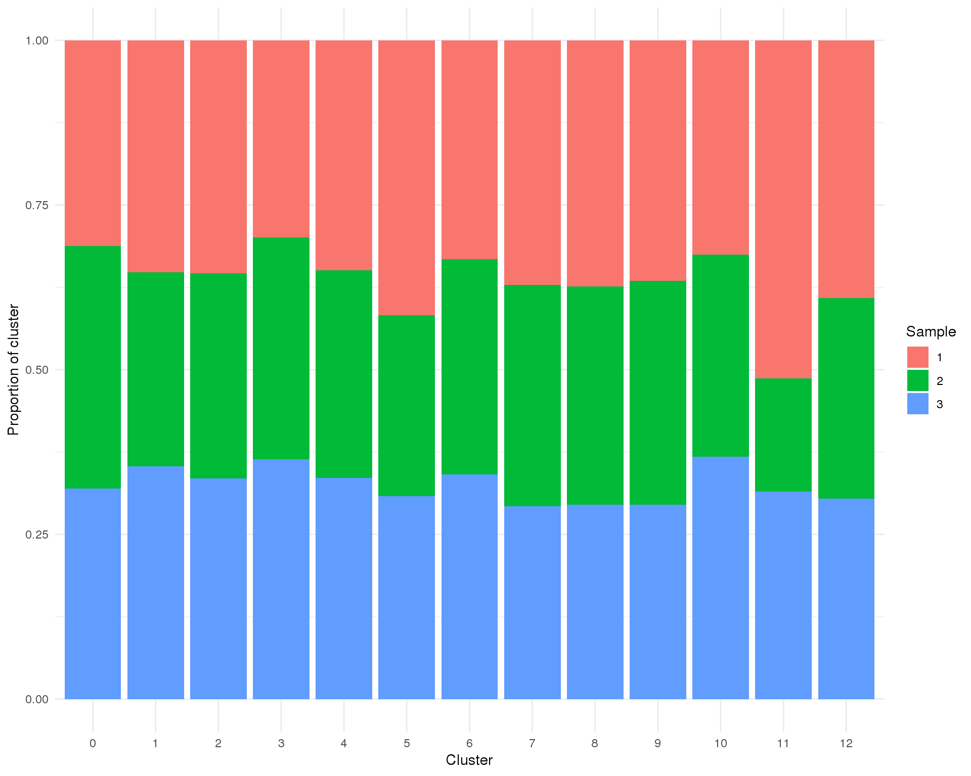
PCA
plotReducedDim(sce, "SeuratPCA", colour_by = "Sample", add_ticks = FALSE,
               point_alpha = 1) +
    scale_fill_discrete() +
    theme_minimal()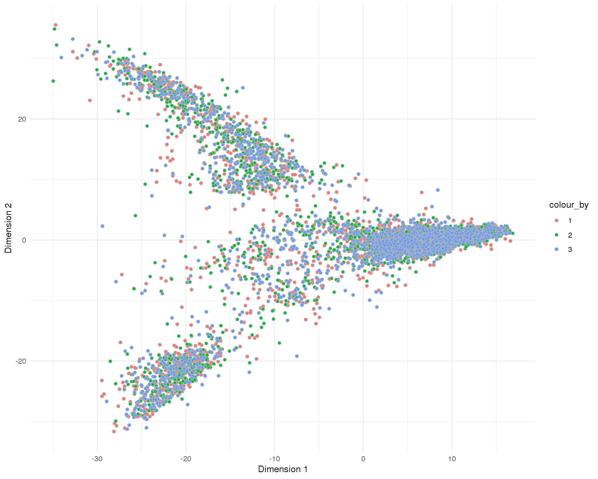
t-SNE
plotReducedDim(sce, "SeuratTSNE", colour_by = "Sample", add_ticks = FALSE,
               point_alpha = 1) +
    scale_fill_discrete() +
    theme_minimal()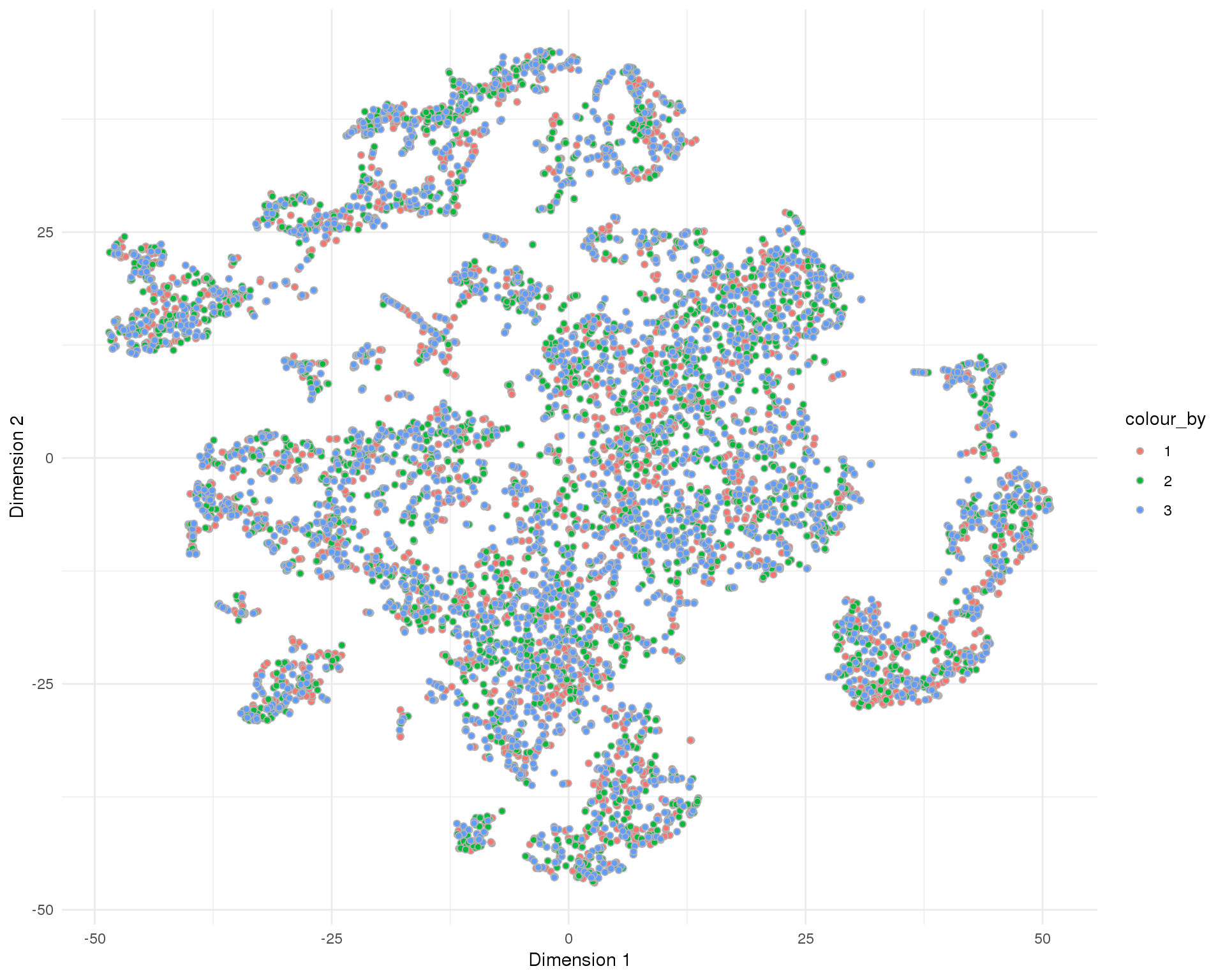
UMAP
plotReducedDim(sce, "SeuratUMAP", colour_by = "Sample", add_ticks = FALSE,
               point_alpha = 1) +
    scale_fill_discrete() +
    theme_minimal()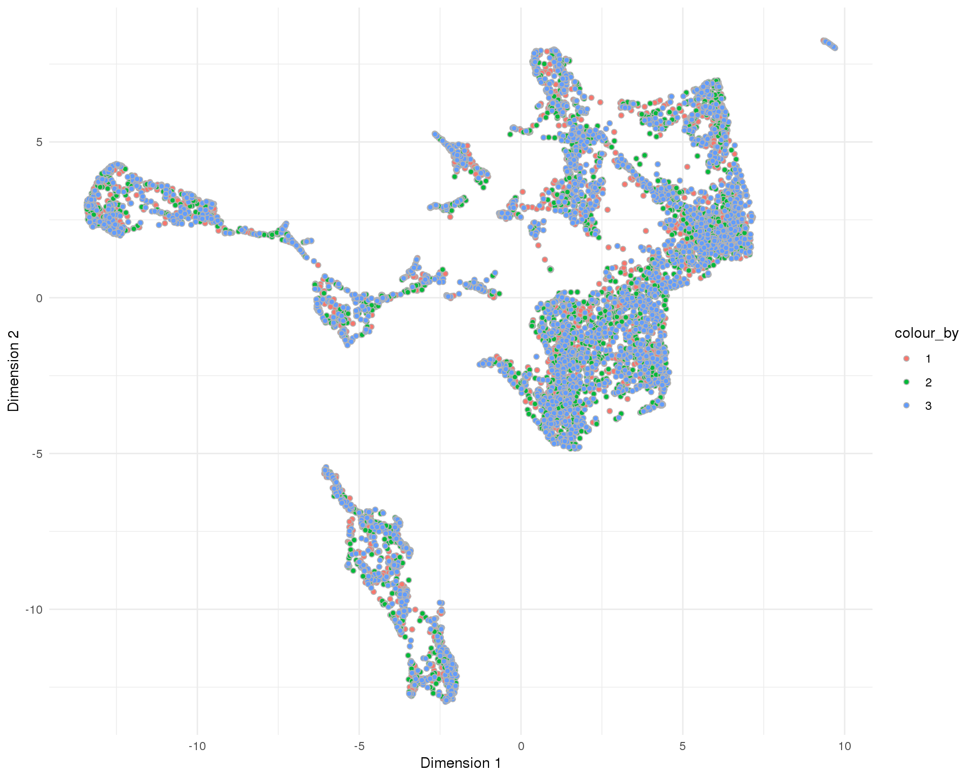
Selection method
Method used to select droplet-containing cells.
Count
ggplot(cell_data, aes(x = Cluster, fill = SelMethod)) +
    geom_bar() +
    theme_minimal()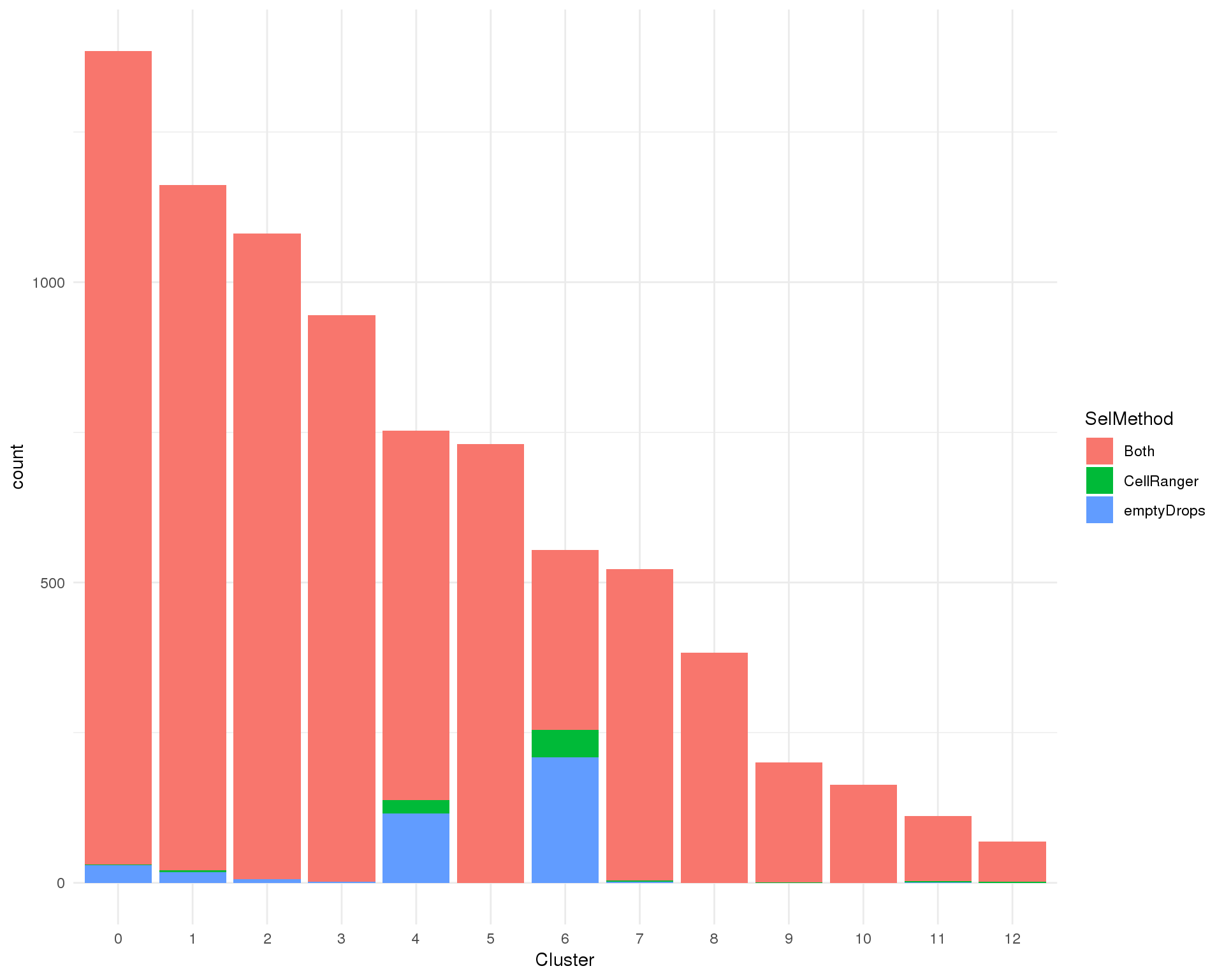
Proportion
plot_data <- cell_data %>%
    group_by(Cluster, SelMethod) %>%
    summarise(Count = n()) %>%
    mutate(Prop = Count / sum(Count))

ggplot(plot_data, aes(x = Cluster, y = Prop, fill = SelMethod)) +
    geom_col() +
    ylab("Proportion of cluster") +
    theme_minimal()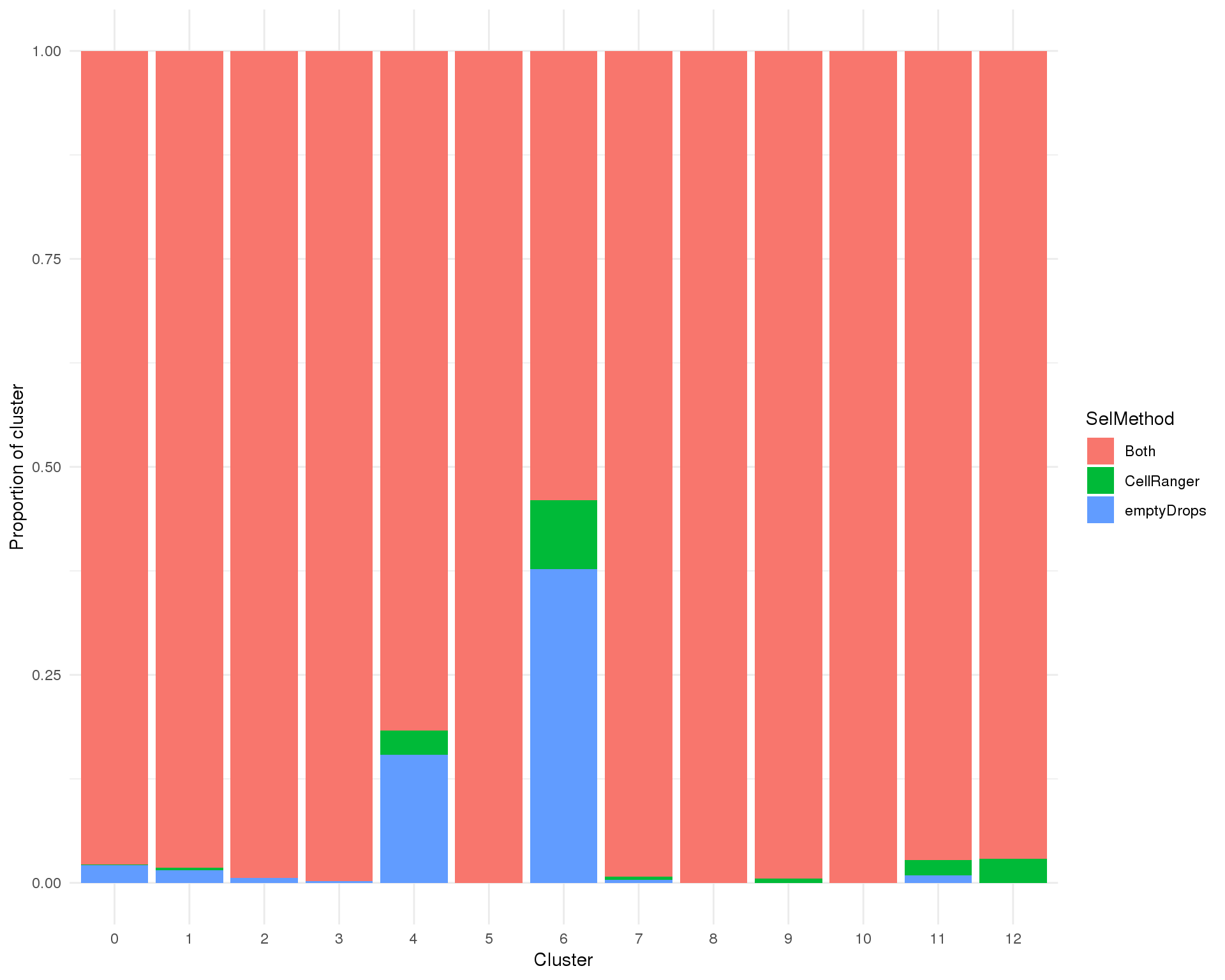
PCA
plotReducedDim(sce, "SeuratPCA", colour_by = "SelMethod", add_ticks = FALSE,
               point_alpha = 1) +
    scale_fill_discrete() +
    theme_minimal()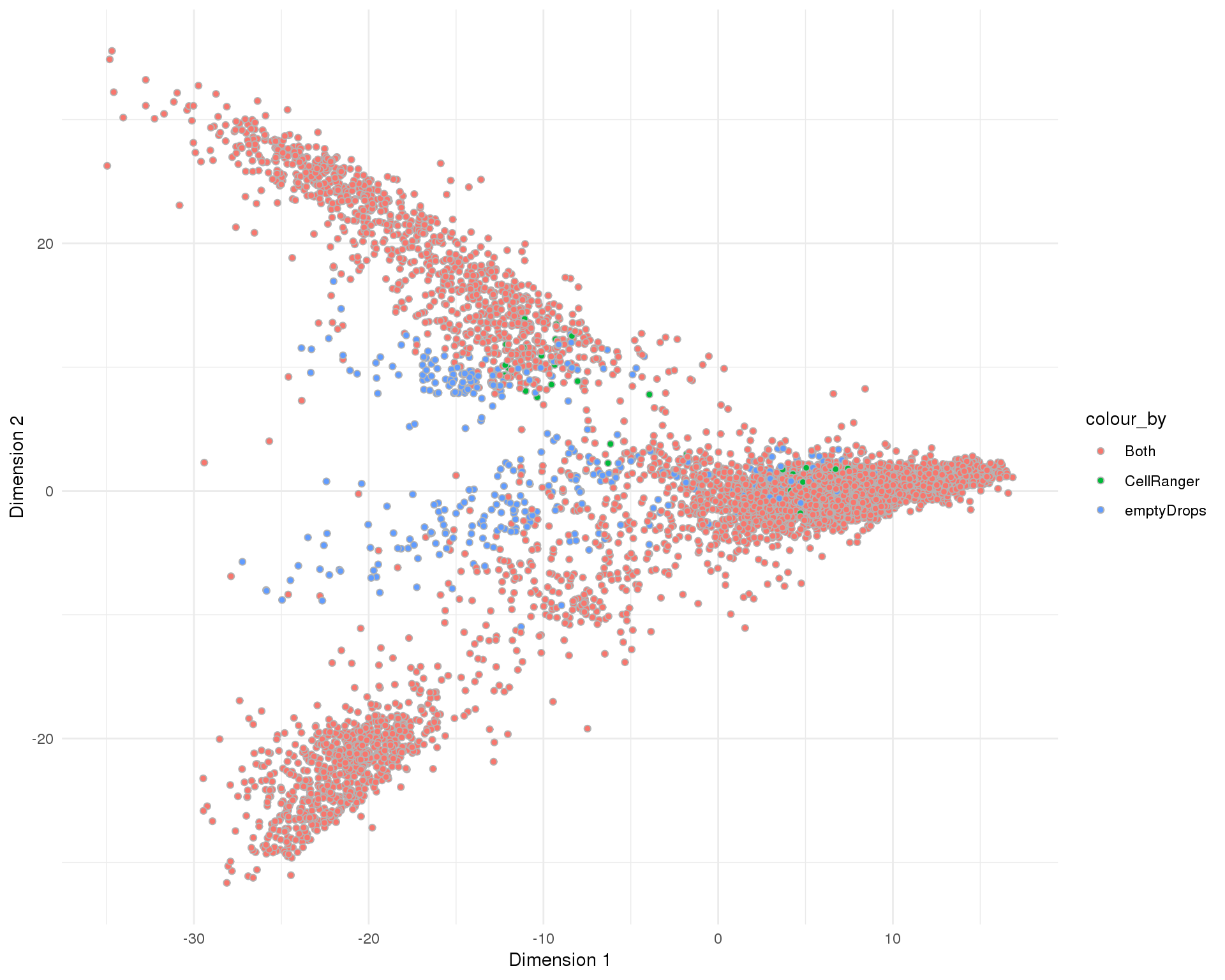
t-SNE
plotReducedDim(sce, "SeuratTSNE", colour_by = "SelMethod", add_ticks = FALSE,
               point_alpha = 1) +
    scale_fill_discrete() +
    theme_minimal()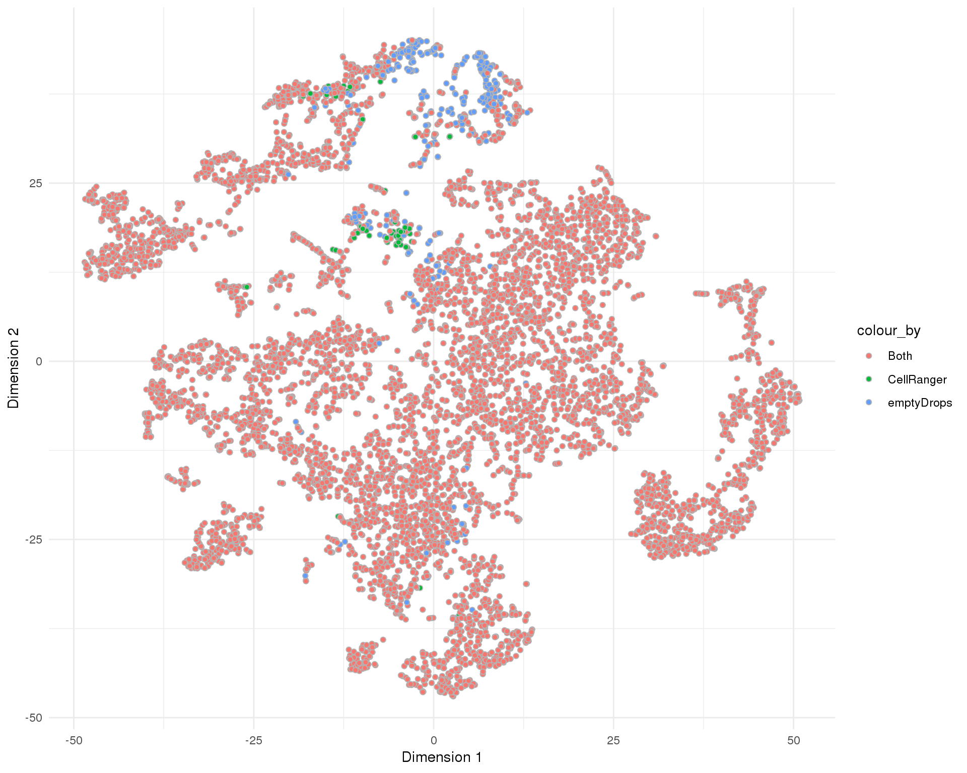
UMAP
plotReducedDim(sce, "SeuratUMAP", colour_by = "SelMethod", add_ticks = FALSE,
               point_alpha = 1) +
    scale_fill_discrete() +
    theme_minimal()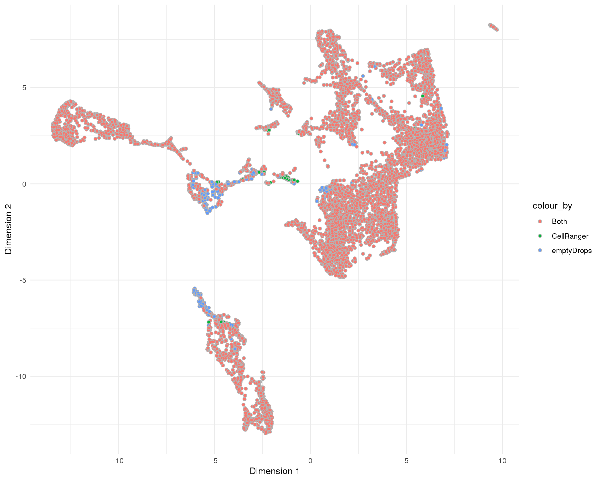
Cell cycle
Cell cycle phases assigned by scran.
Count
ggplot(cell_data, aes(x = Cluster, fill = CellCycle)) +
    geom_bar() +
    theme_minimal()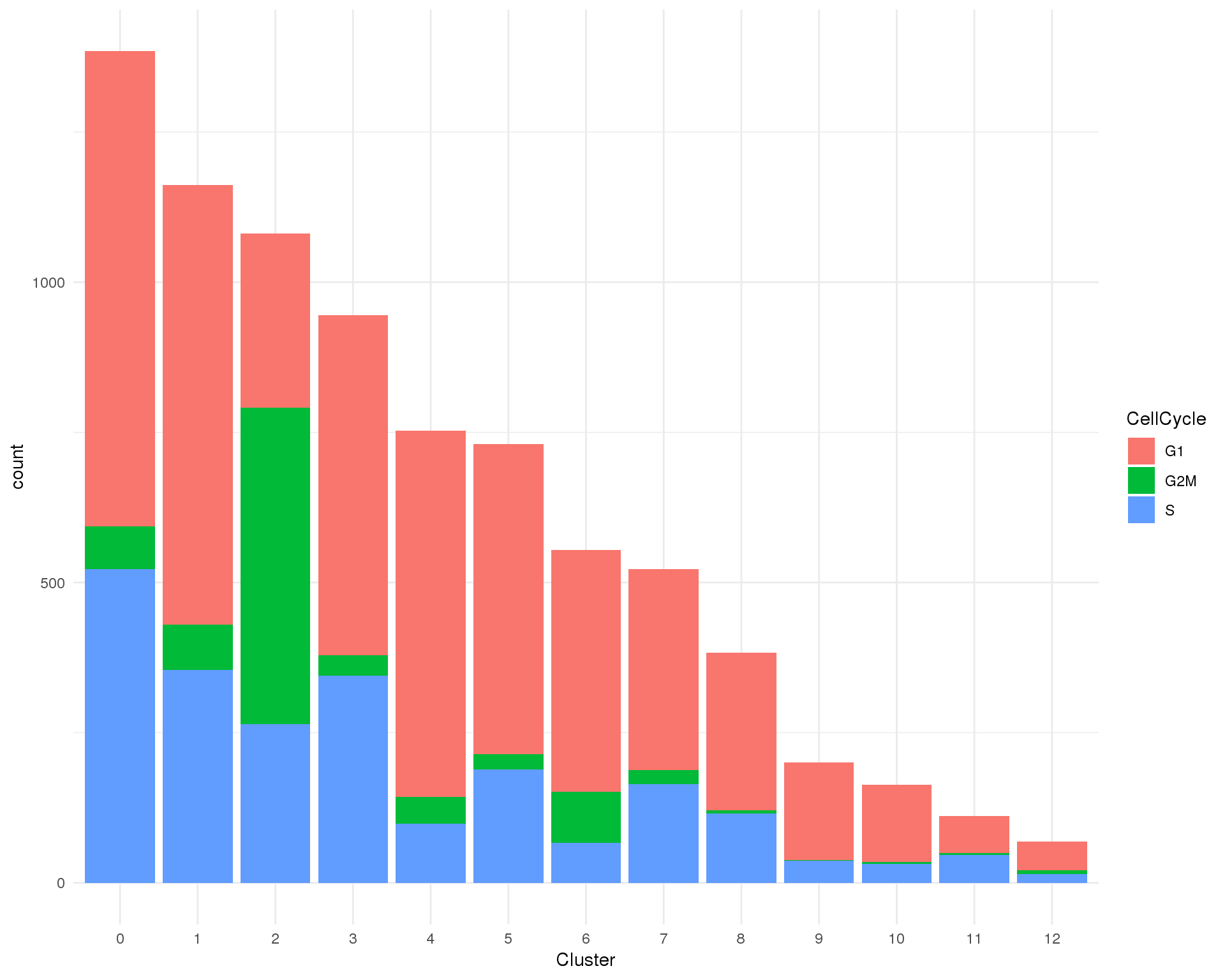
Proportion
plot_data <- cell_data %>%
    group_by(Cluster, CellCycle) %>%
    summarise(Count = n()) %>%
    mutate(Prop = Count / sum(Count))

ggplot(plot_data, aes(x = Cluster, y = Prop, fill = CellCycle)) +
    geom_col() +
    ylab("Proportion of cluster") +
    theme_minimal()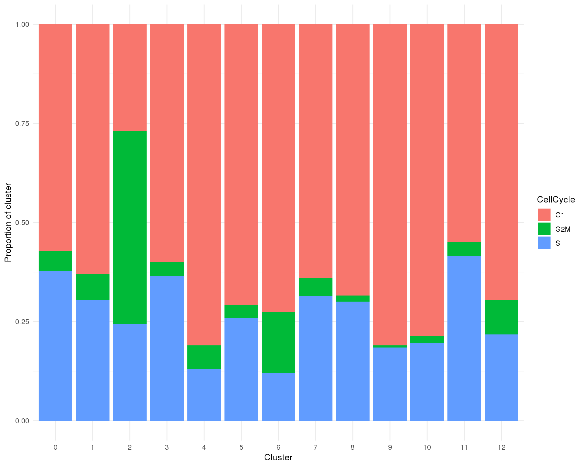
PCA
plotReducedDim(sce, "SeuratPCA", colour_by = "CellCycle", add_ticks = FALSE,
               point_alpha = 1) +
    scale_fill_discrete() +
    theme_minimal()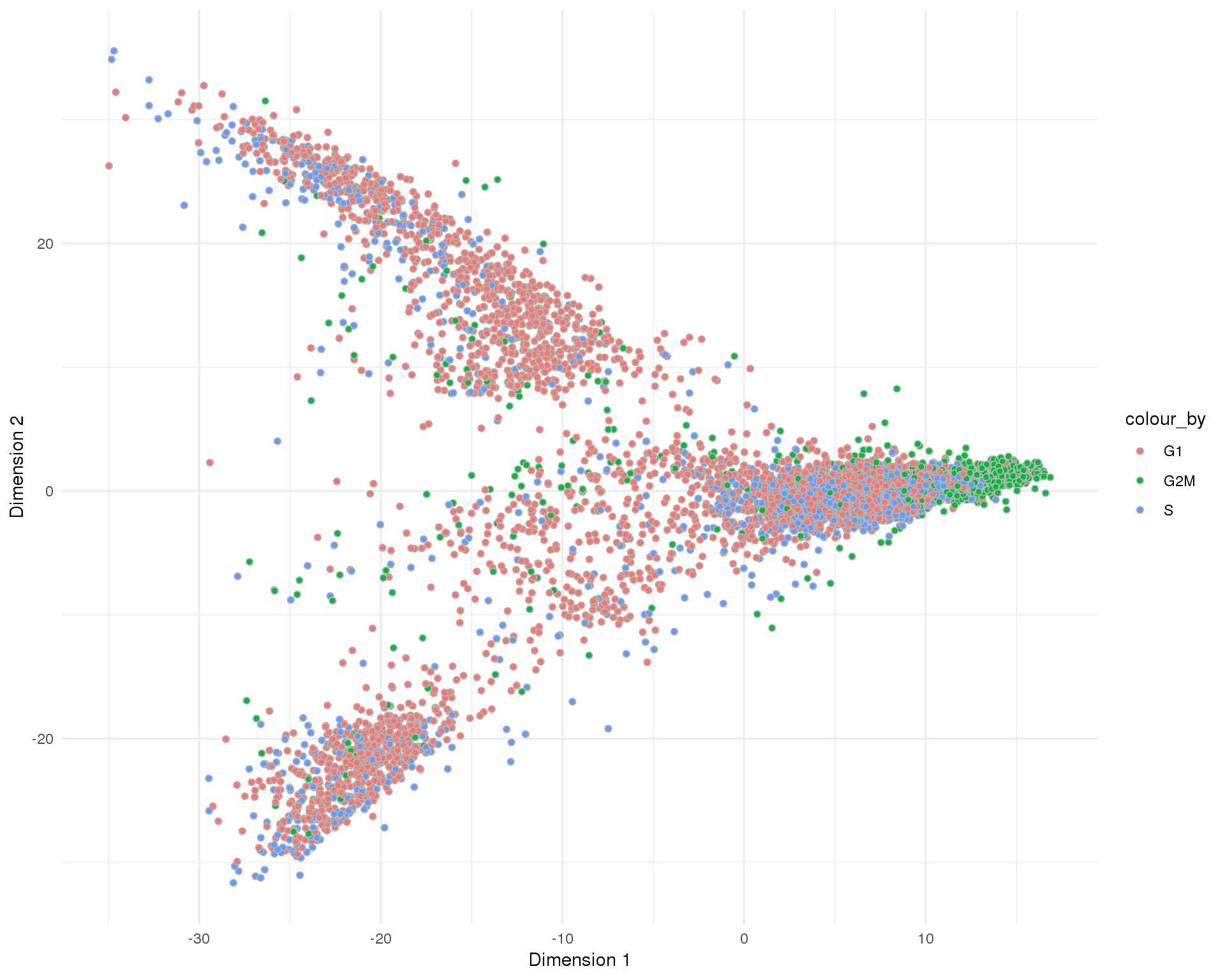
t-SNE
plotReducedDim(sce, "SeuratTSNE", colour_by = "CellCycle", add_ticks = FALSE,
               point_alpha = 1) +
    scale_fill_discrete() +
    theme_minimal()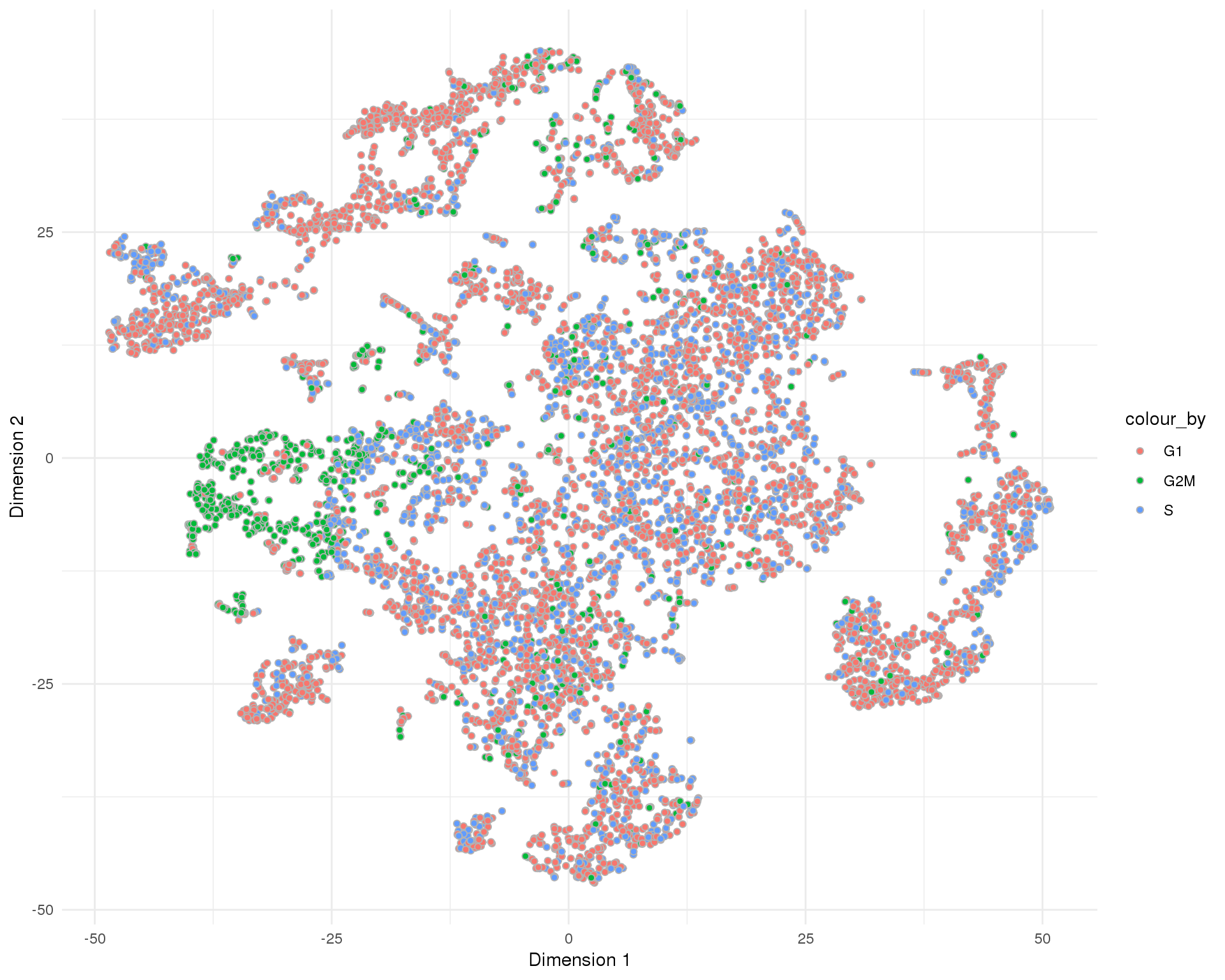
UMAP
plotReducedDim(sce, "SeuratUMAP", colour_by = "CellCycle", add_ticks = FALSE,
               point_alpha = 1) +
    scale_fill_discrete() +
    theme_minimal()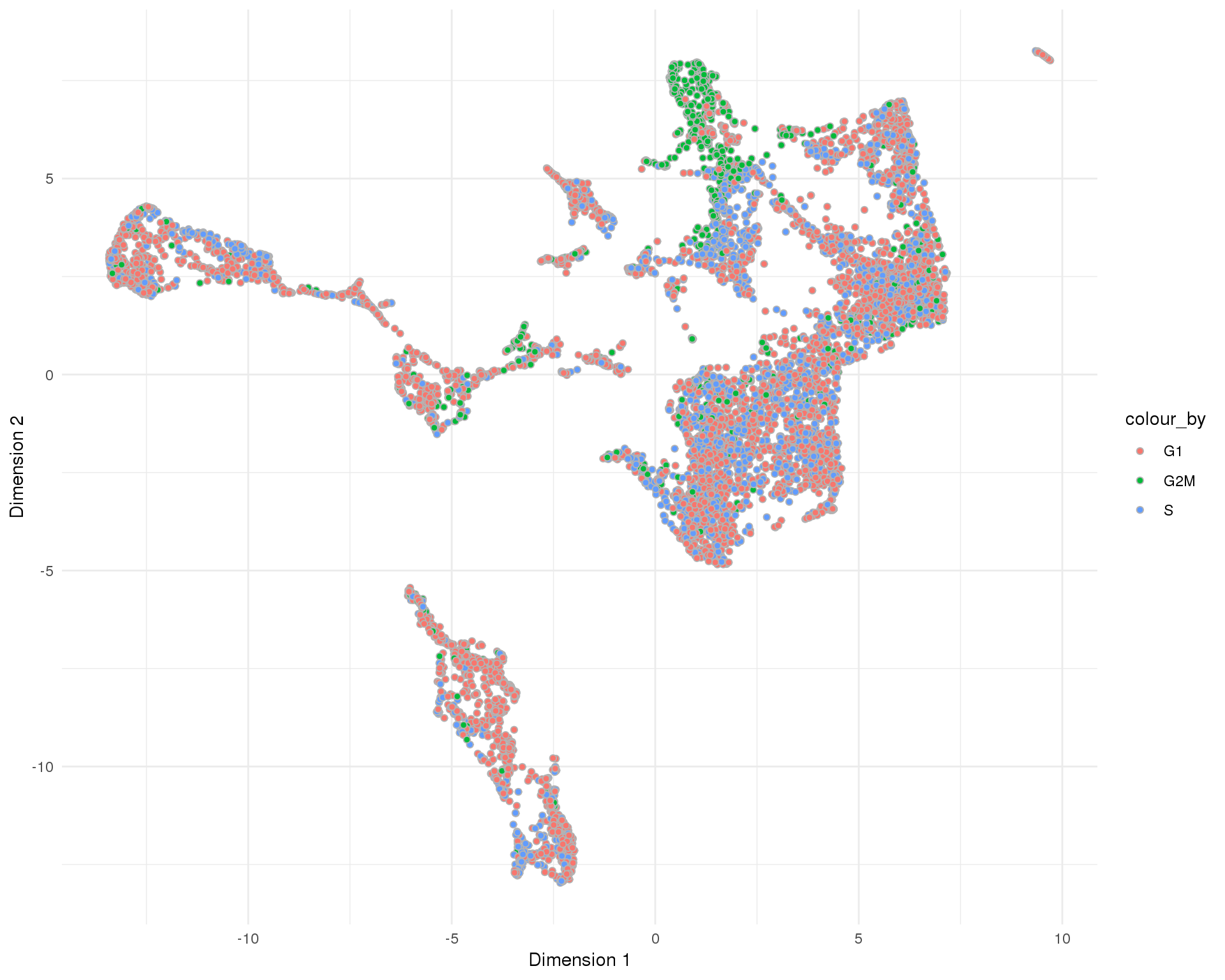
Total counts
Total counts per cell.
Distribution
ggplot(cell_data, aes(x = Cluster, y = log10_total_counts)) +
    geom_violin() +
    geom_sina(aes(colour = Cluster), size = 0.5) +
    theme_minimal() +
    theme(legend.position = "none")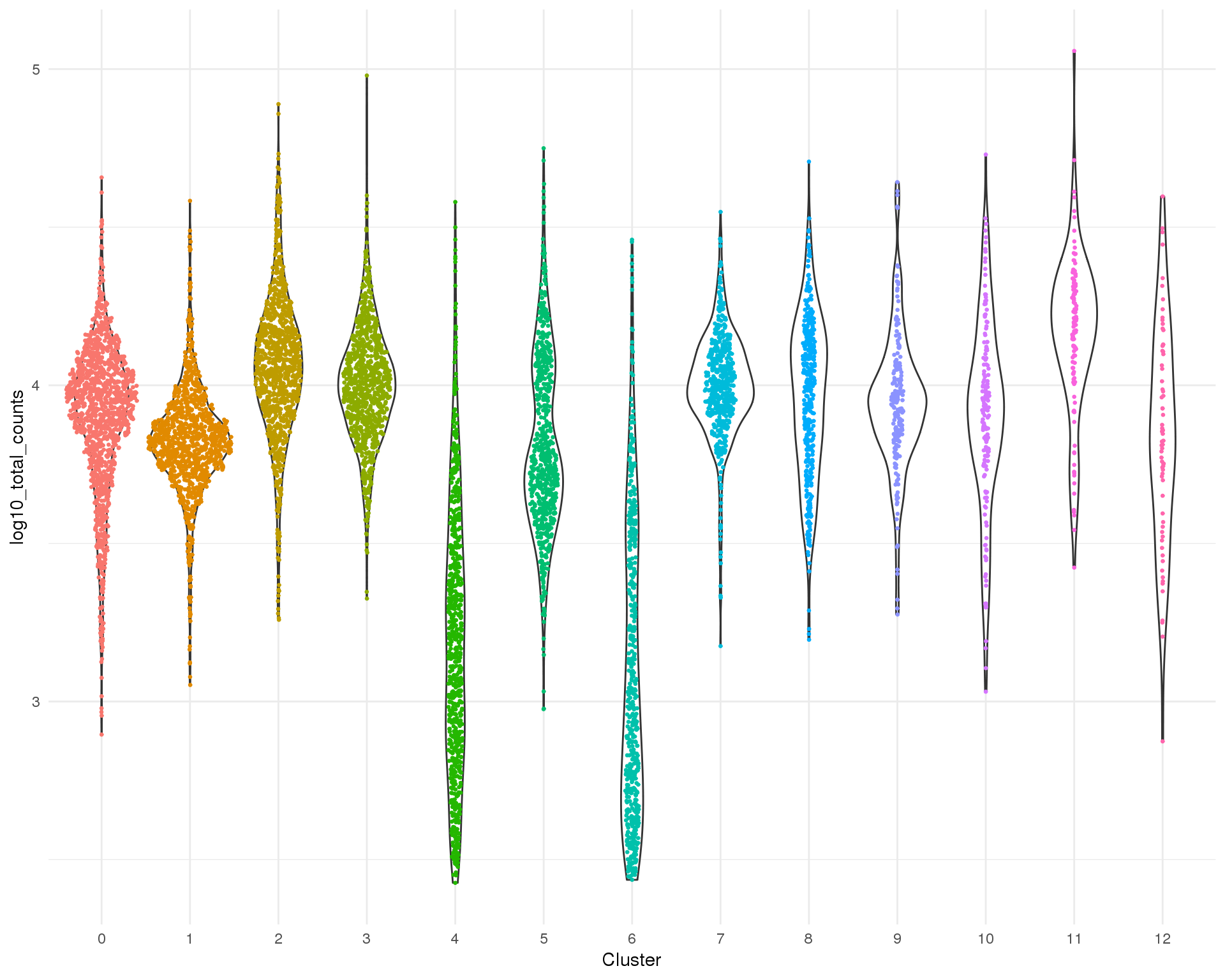
PCA
plotReducedDim(sce, "SeuratPCA", colour_by = "log10_total_counts",
               add_ticks = FALSE, point_alpha = 1) +
    scale_fill_viridis_c() +
    theme_minimal()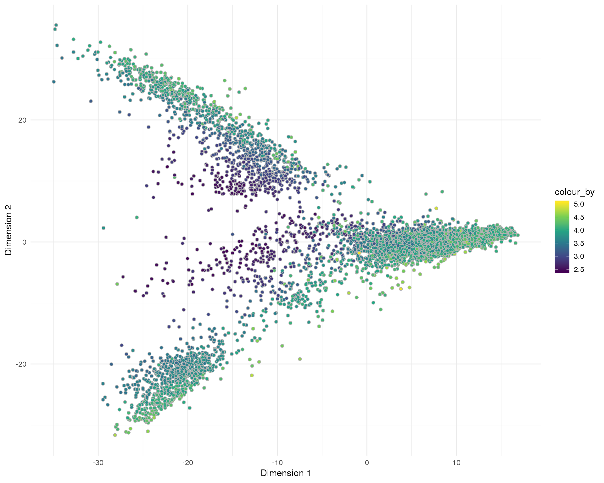
t-SNE
plotReducedDim(sce, "SeuratTSNE", colour_by = "log10_total_counts",
               add_ticks = FALSE, point_alpha = 1) +
    scale_fill_viridis_c() +
    theme_minimal()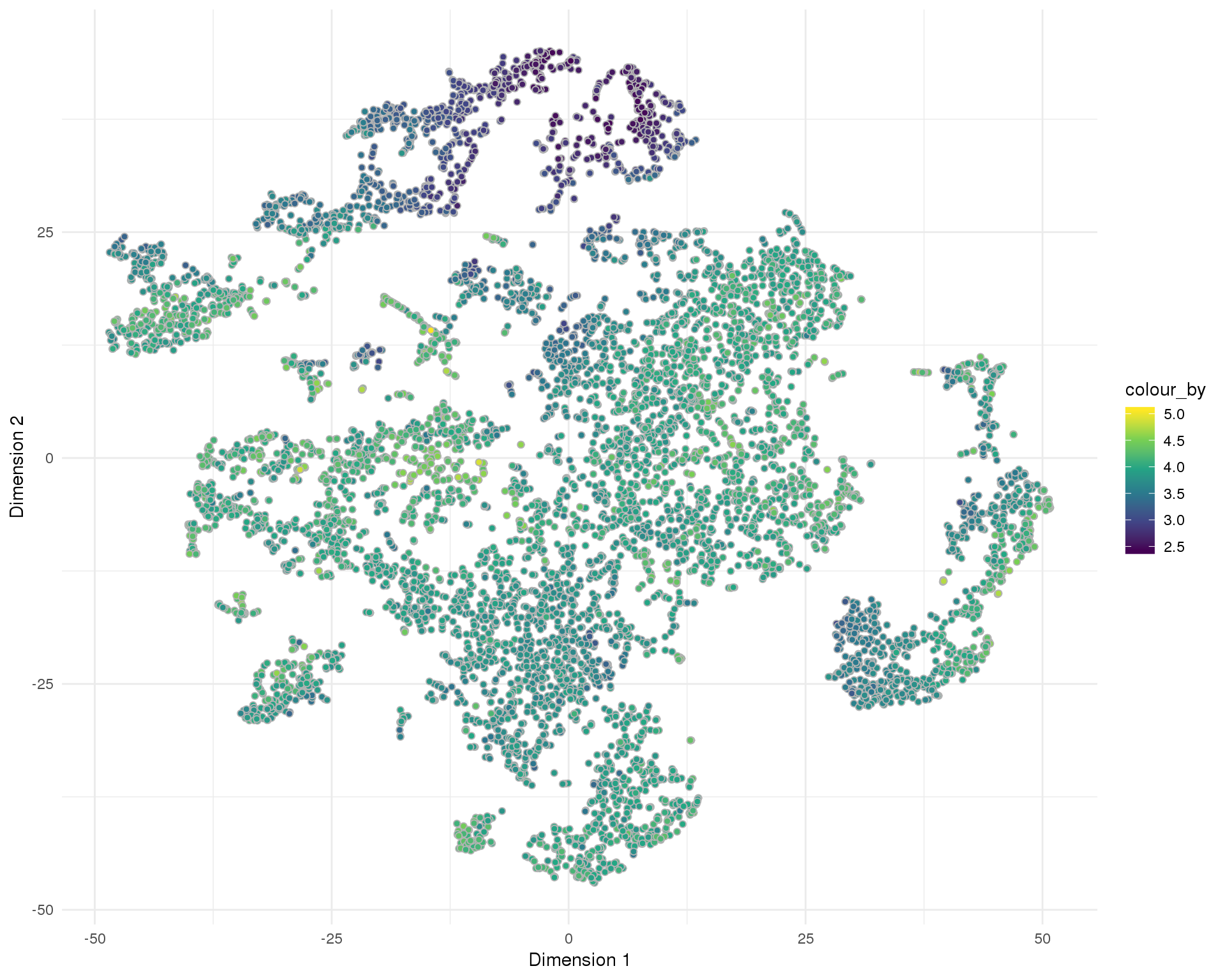
UMAP
plotReducedDim(sce, "SeuratUMAP", colour_by = "log10_total_counts",
               add_ticks = FALSE, point_alpha = 1) +
    scale_fill_viridis_c() +
    theme_minimal()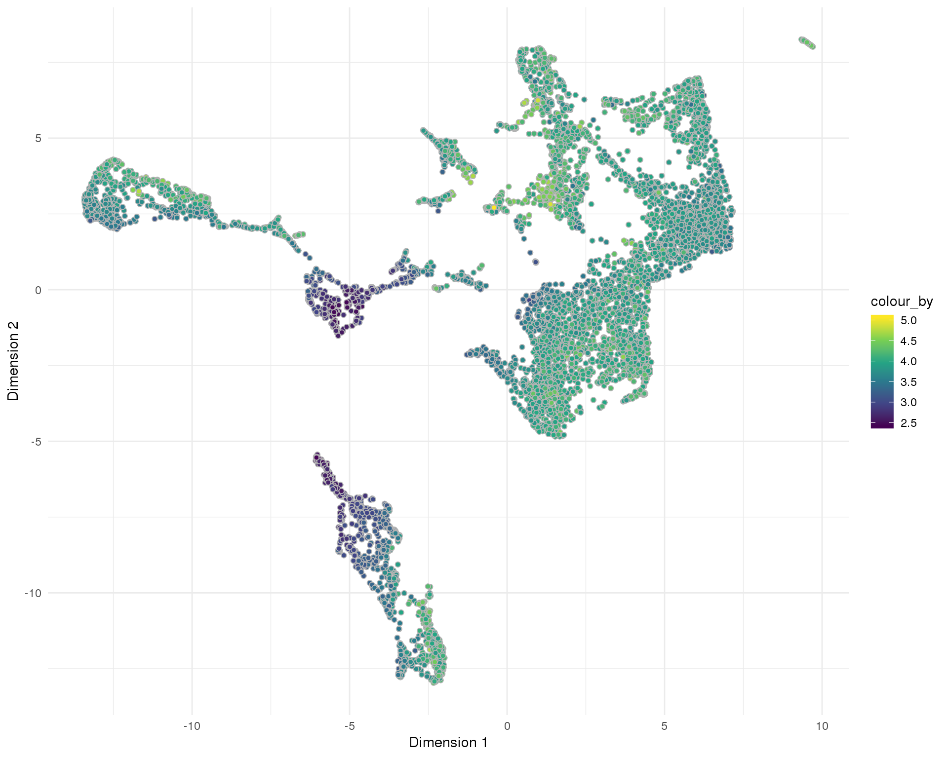
Total features
Total number of expressed features per cell.
Distribution
ggplot(cell_data, aes(x = Cluster, y = log10_total_features_by_counts)) +
    geom_violin() +
    geom_sina(aes(colour = Cluster), size = 0.5) +
    theme_minimal() +
    theme(legend.position = "none")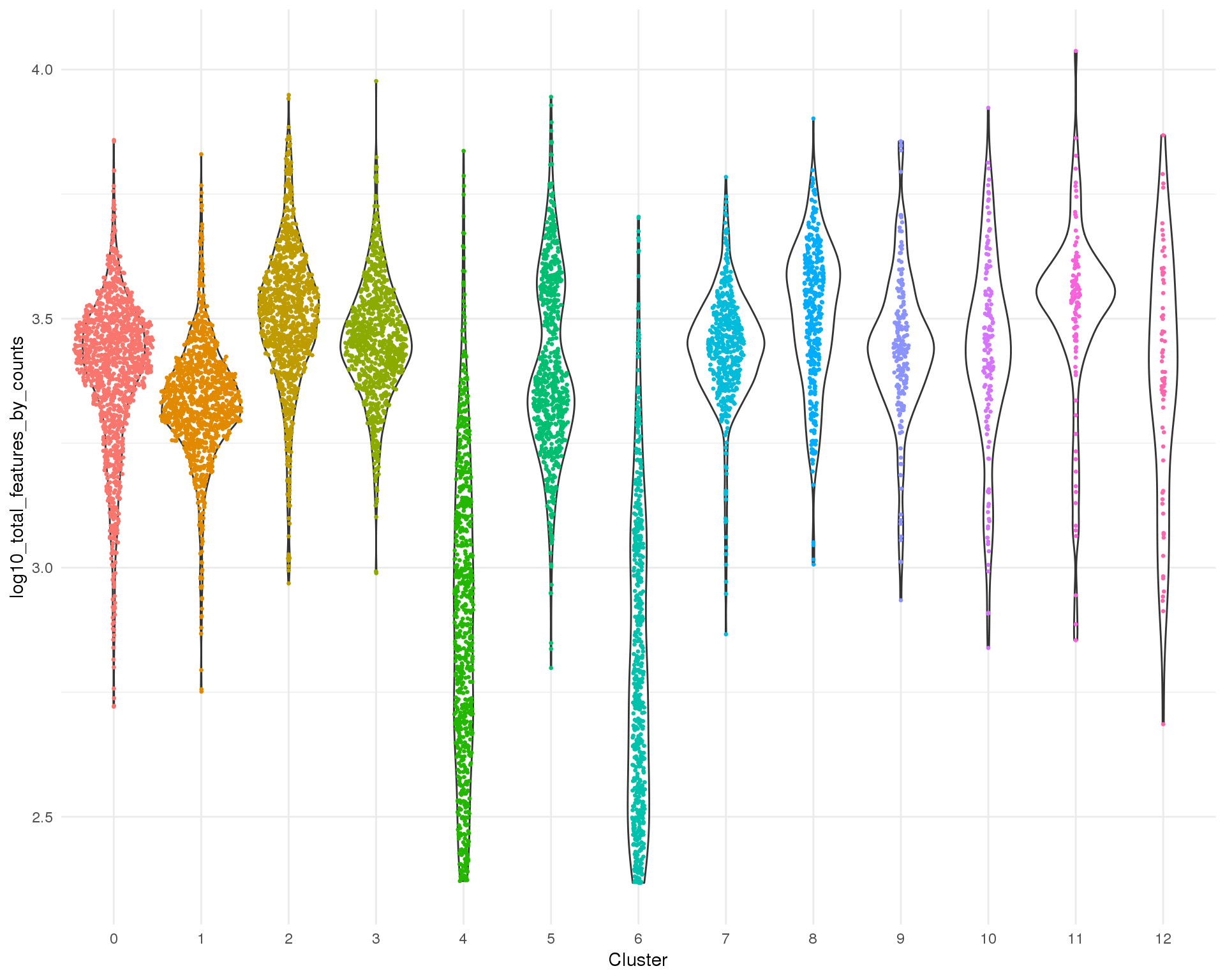
PCA
plotReducedDim(sce, "SeuratPCA", colour_by = "log10_total_features_by_counts",
               add_ticks = FALSE, point_alpha = 1) +
    scale_fill_viridis_c() +
    theme_minimal()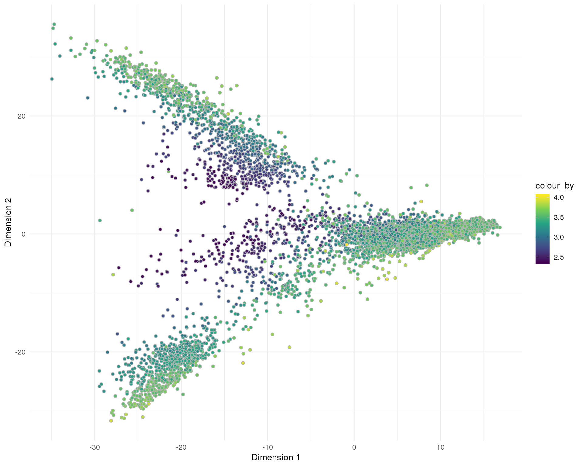
t-SNE
plotReducedDim(sce, "SeuratTSNE", colour_by = "log10_total_features_by_counts",
               add_ticks = FALSE, point_alpha = 1) +
    scale_fill_viridis_c() +
    theme_minimal()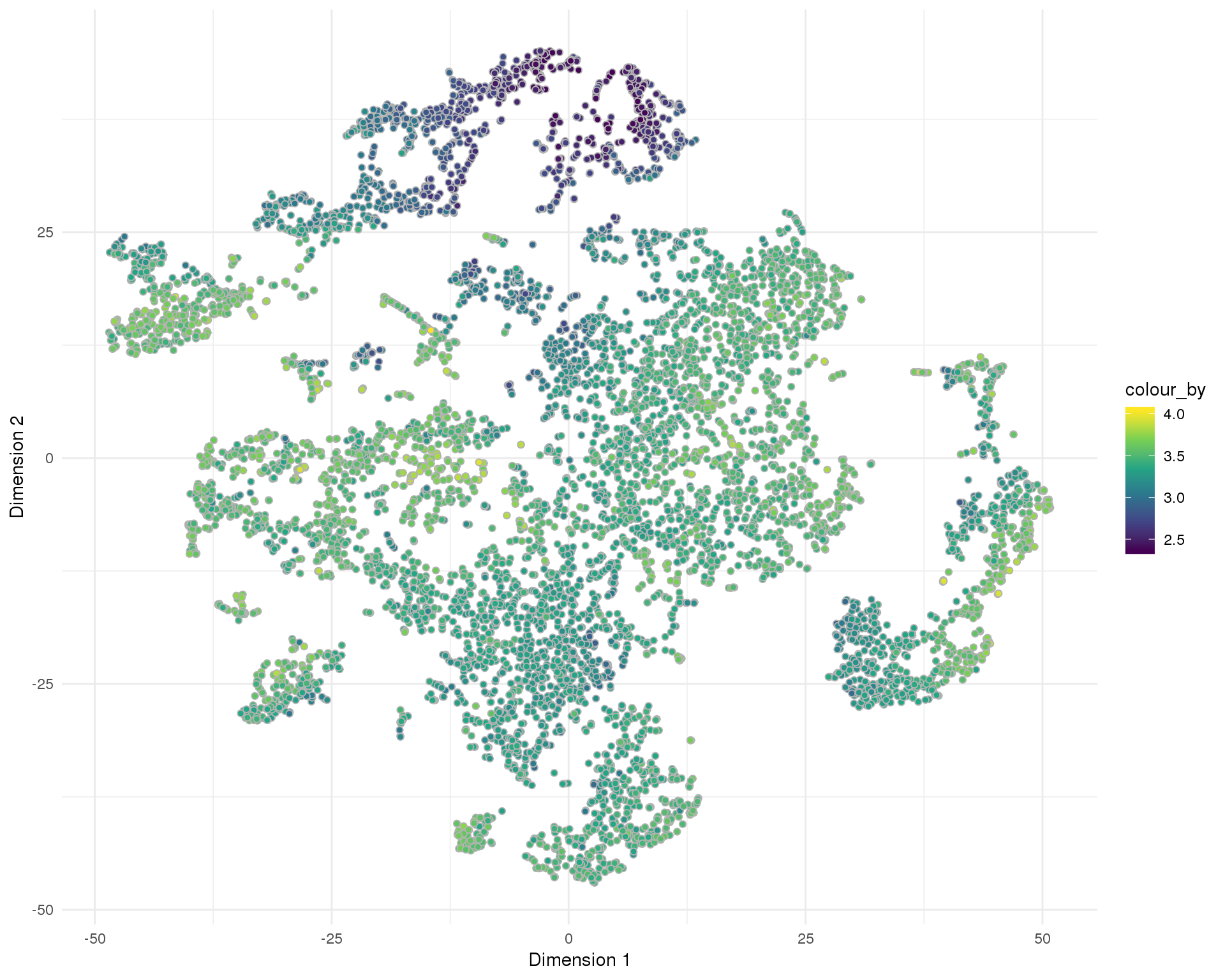
UMAP
plotReducedDim(sce, "SeuratUMAP", colour_by = "log10_total_features_by_counts",
               add_ticks = FALSE, point_alpha = 1) +
    scale_fill_viridis_c() +
    theme_minimal()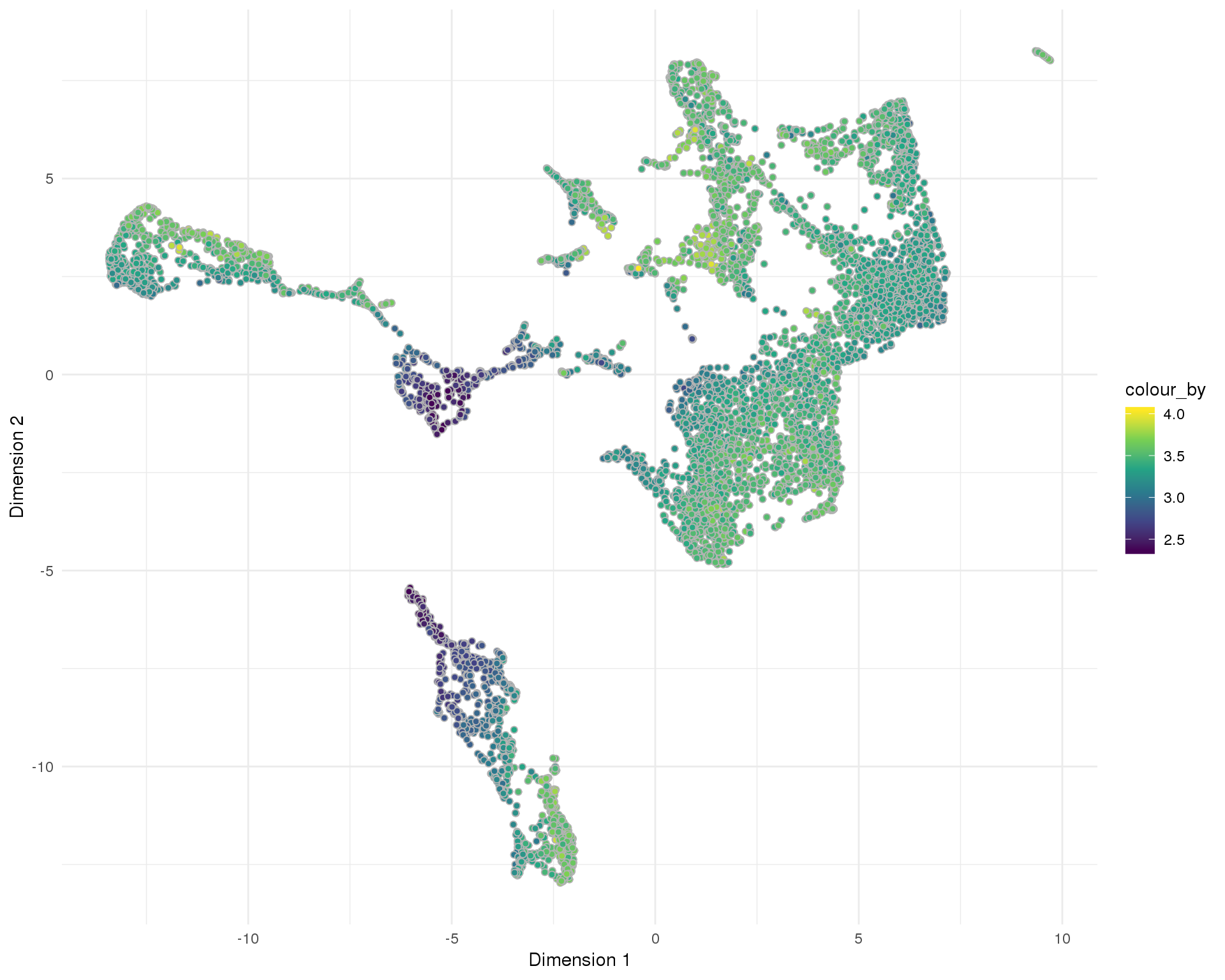
Mitochondrial genes
Percentage of counts assigned to mitochondrial genes per cell.
Distribution
ggplot(cell_data, aes(x = Cluster, y = pct_counts_MT)) +
    geom_violin() +
    geom_sina(aes(colour = Cluster), size = 0.5) +
    theme_minimal() +
    theme(legend.position = "none")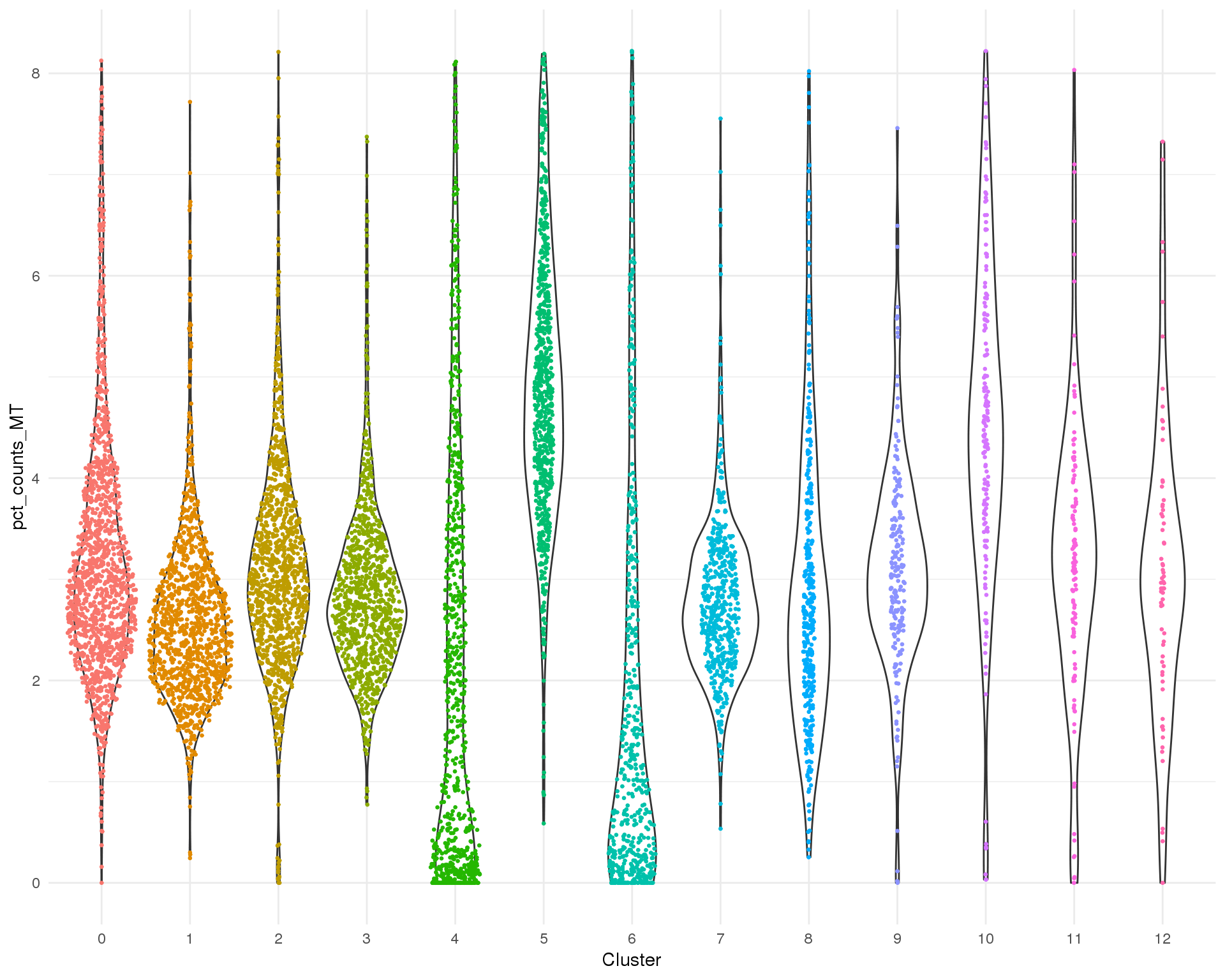
PCA
plotReducedDim(sce, "SeuratPCA", colour_by = "pct_counts_MT",
               add_ticks = FALSE, point_alpha = 1) +
    scale_fill_viridis_c() +
    theme_minimal()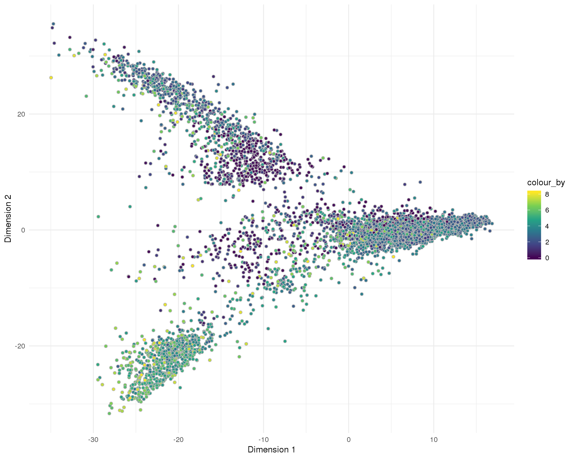
t-SNE
plotReducedDim(sce, "SeuratTSNE", colour_by = "pct_counts_MT",
               add_ticks = FALSE, point_alpha = 1) +
    scale_fill_viridis_c() +
    theme_minimal()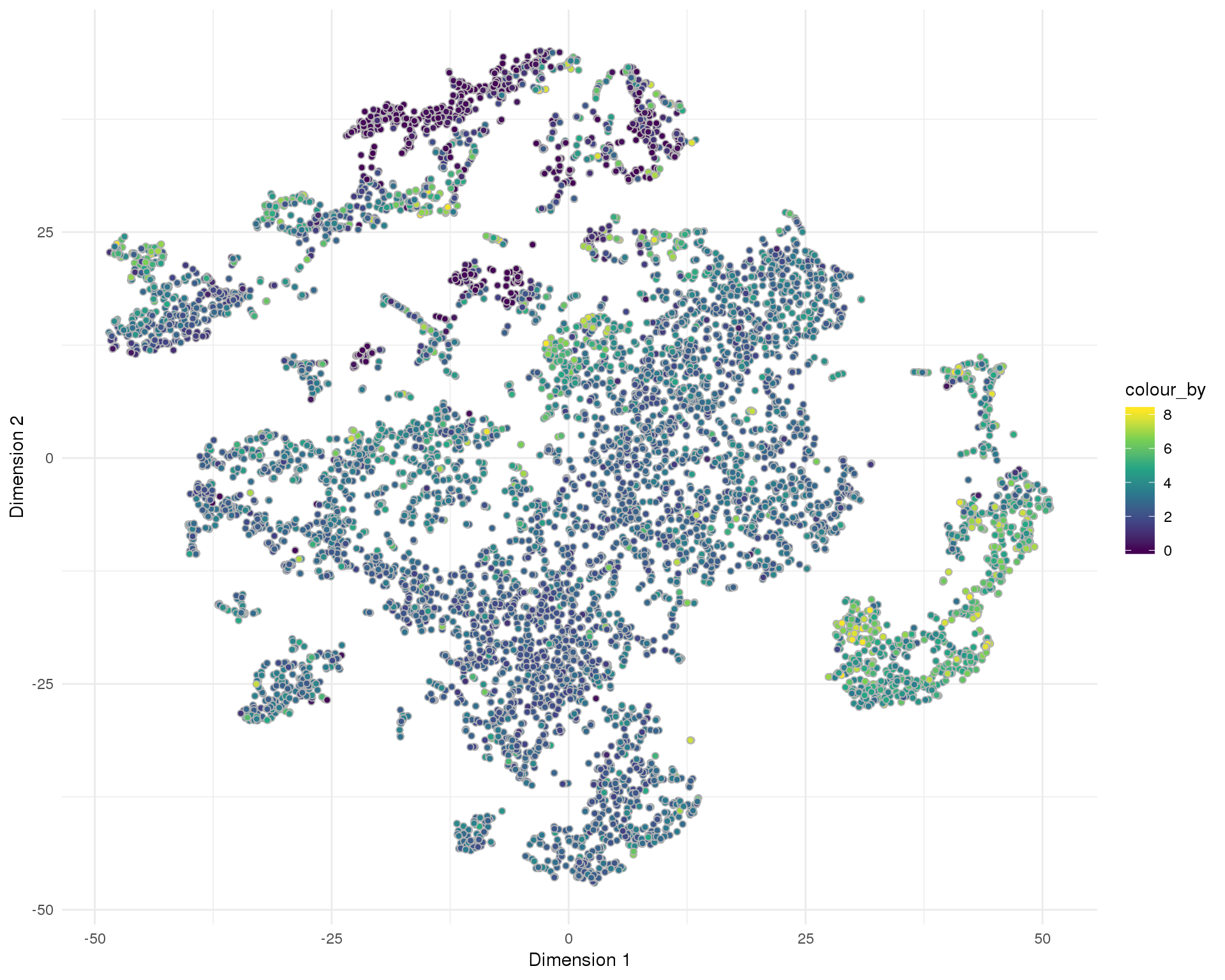
UMAP
plotReducedDim(sce, "SeuratUMAP", colour_by = "pct_counts_MT",
               add_ticks = FALSE, point_alpha = 1) +
    scale_fill_viridis_c() +
    theme_minimal()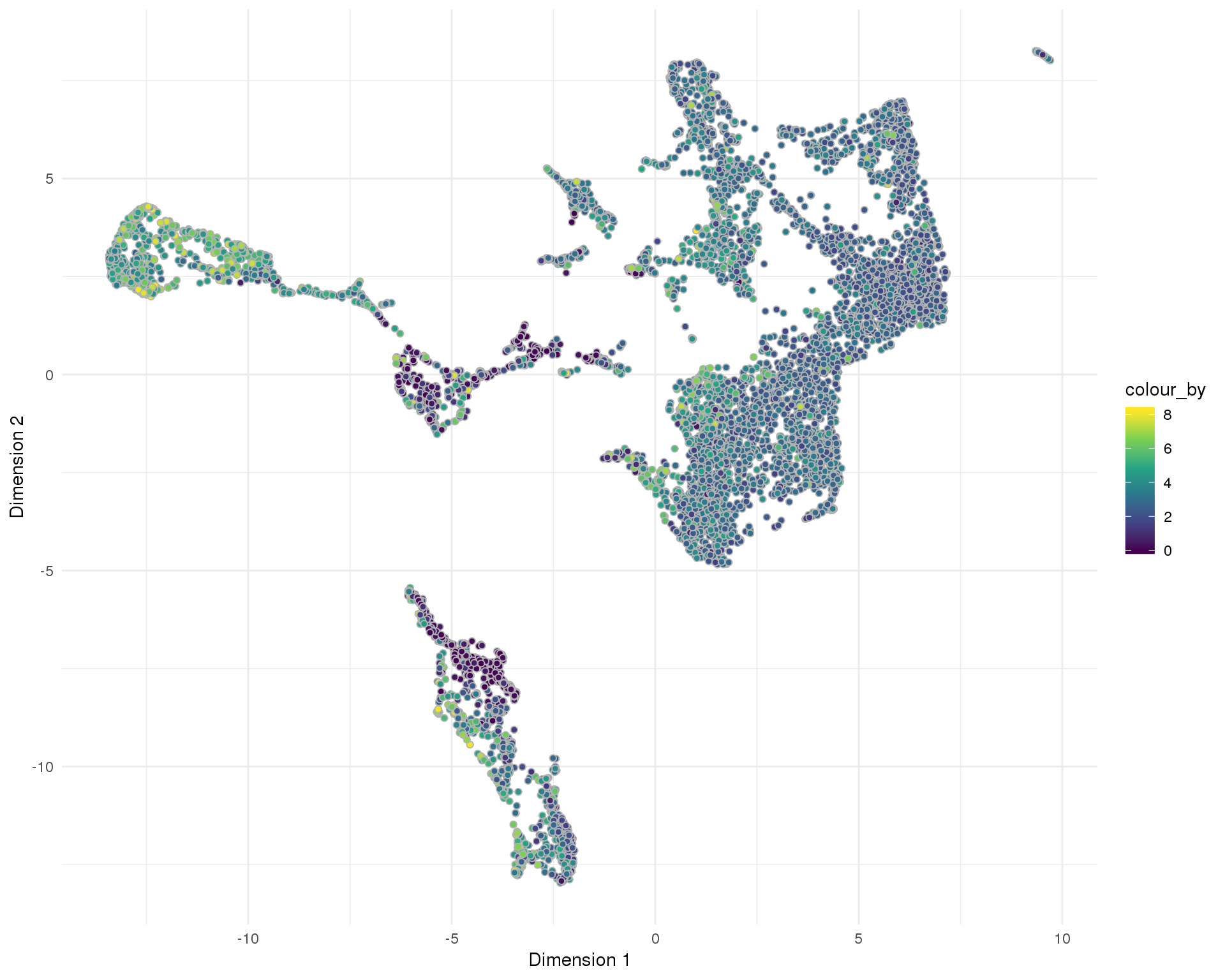
Doublet score
Doublet score assigned by scran per cell.
Distribution
ggplot(cell_data, aes(x = Cluster, y = DoubletScore)) +
    geom_violin() +
    geom_sina(aes(colour = Cluster), size = 0.5) +
    theme_minimal() +
    theme(legend.position = "none")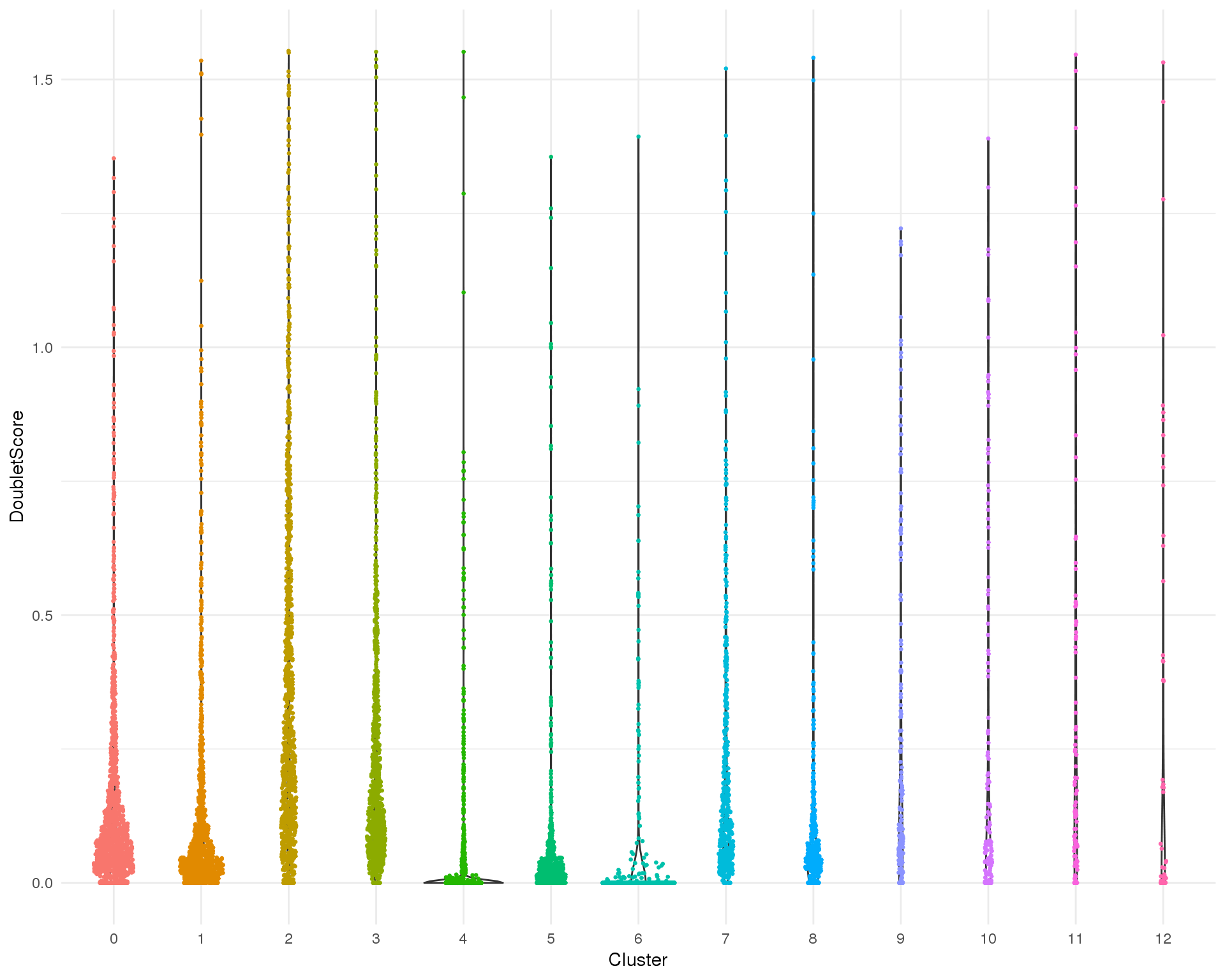
PCA
plotReducedDim(sce, "SeuratPCA", colour_by = "DoubletScore",
               add_ticks = FALSE, point_alpha = 1) +
    scale_fill_viridis_c() +
    theme_minimal()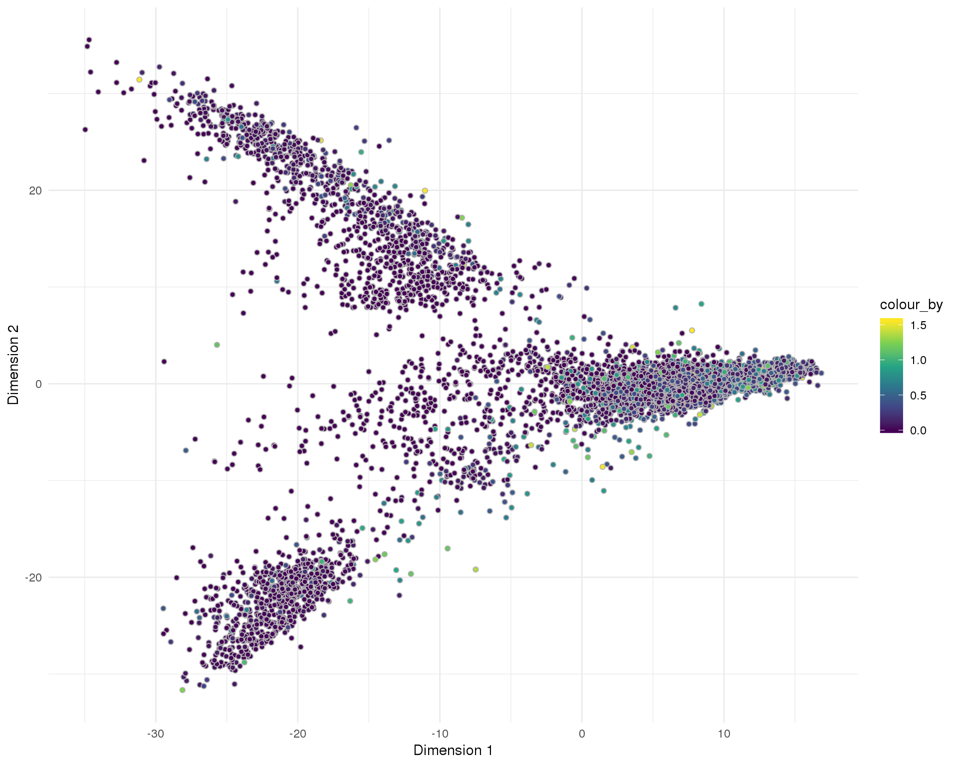
t-SNE
plotReducedDim(sce, "SeuratTSNE", colour_by = "DoubletScore",
               add_ticks = FALSE, point_alpha = 1) +
    scale_fill_viridis_c() +
    theme_minimal()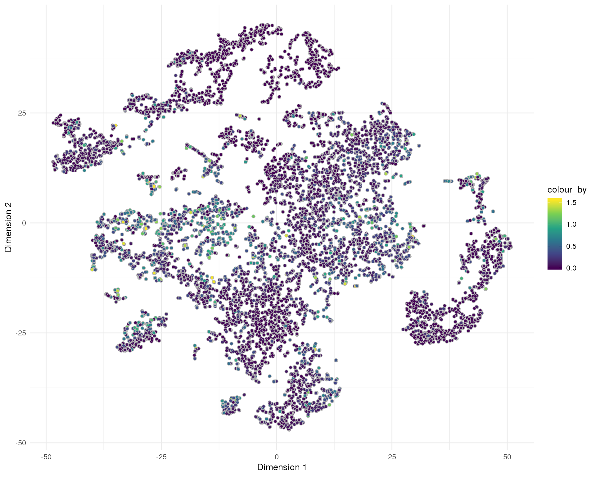
UMAP
plotReducedDim(sce, "SeuratUMAP", colour_by = "DoubletScore",
               add_ticks = FALSE, point_alpha = 1) +
    scale_fill_viridis_c() +
    theme_minimal()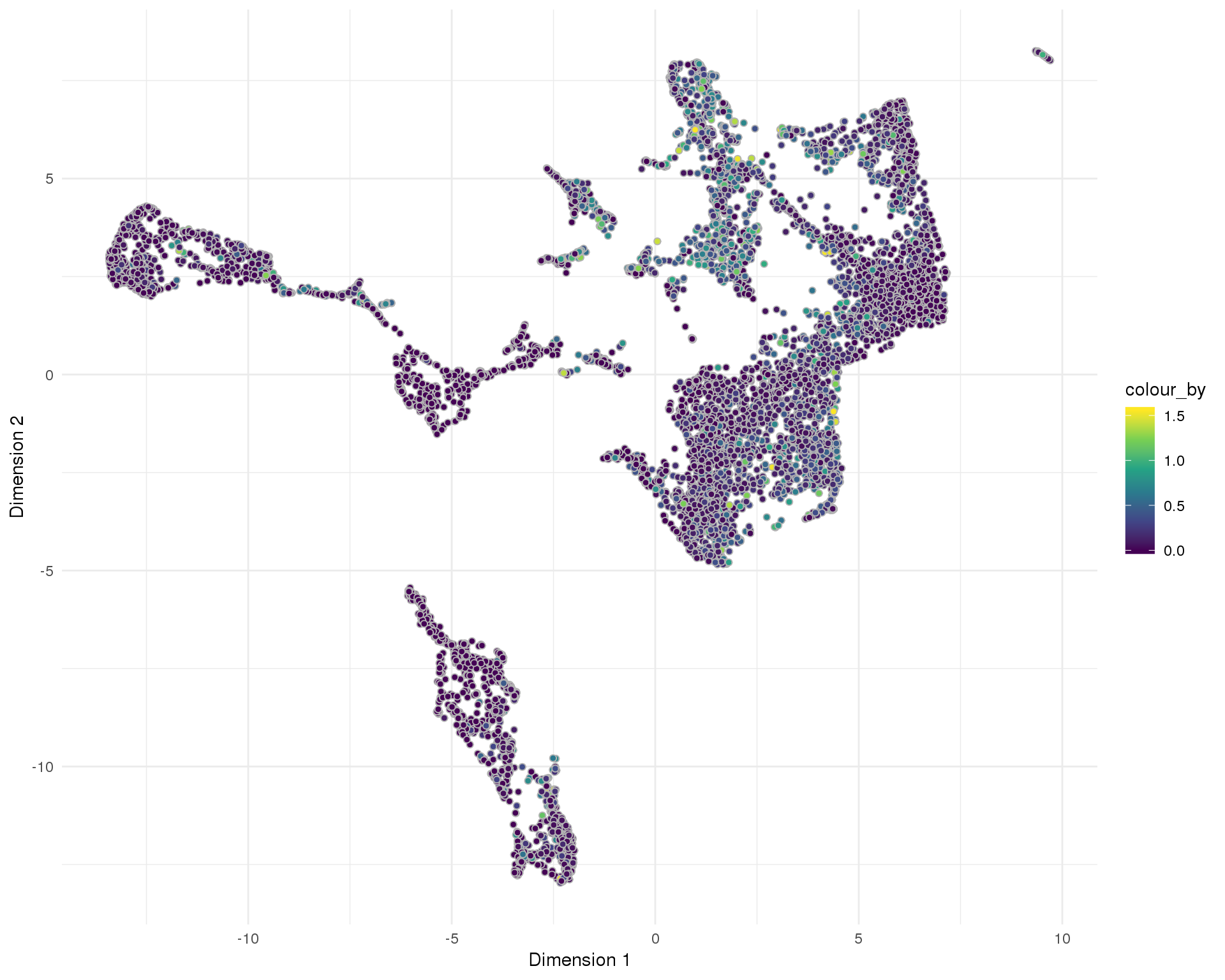
Comparison
Because we have previously published an analysis of this dataset we can check to see how similar these clusters are to what we observed previously and whether the different decisions we have made have significantly changed the results.
assignments <- read_csv(here::here("data/published/cluster_assignments.csv"),
                        col_types = cols(.default = col_character())) %>%
    filter(Dataset == "Organoid123") %>%
    mutate(BarcodeSample = paste(Barcode, Sample, sep = "-")) %>%
    select(BarcodeSample, PubCluster = Cluster) %>%
    mutate(PubCluster = factor(
        PubCluster,
        levels = as.character(0:12),
        labels = c("O0 (Stroma)", "O1 (Stroma)", "O2 (Podocyte)",
                   "O3 (Stroma)", "O4 (Cell cycle)", "O5 (Endothelium)",
                   "O6 (Cell cycle)", "O7 (Stroma)", "O8 (Glial)",
                   "O9 (Epithelium)", "010 (Muscle progenitor)",
                   "O11 (Neural progenitor)", "O12 (Endothelium)")
    ))

cell_data <- cell_data %>%
    mutate(BarcodeSample = paste(Barcode, Sample, sep = "-")) %>%
    left_join(assignments, by = "BarcodeSample")
First let’s look at how many of the cells in each cluster were present in our previous analysis:
plot_data <- cell_data %>%
    mutate(Present = !is.na(PubCluster)) %>%
    group_by(Cluster) %>%
    summarise(PropPresent = sum(Present) / n())

ggplot(plot_data, aes(x = Cluster, y = PropPresent, fill = Cluster)) +
    geom_col()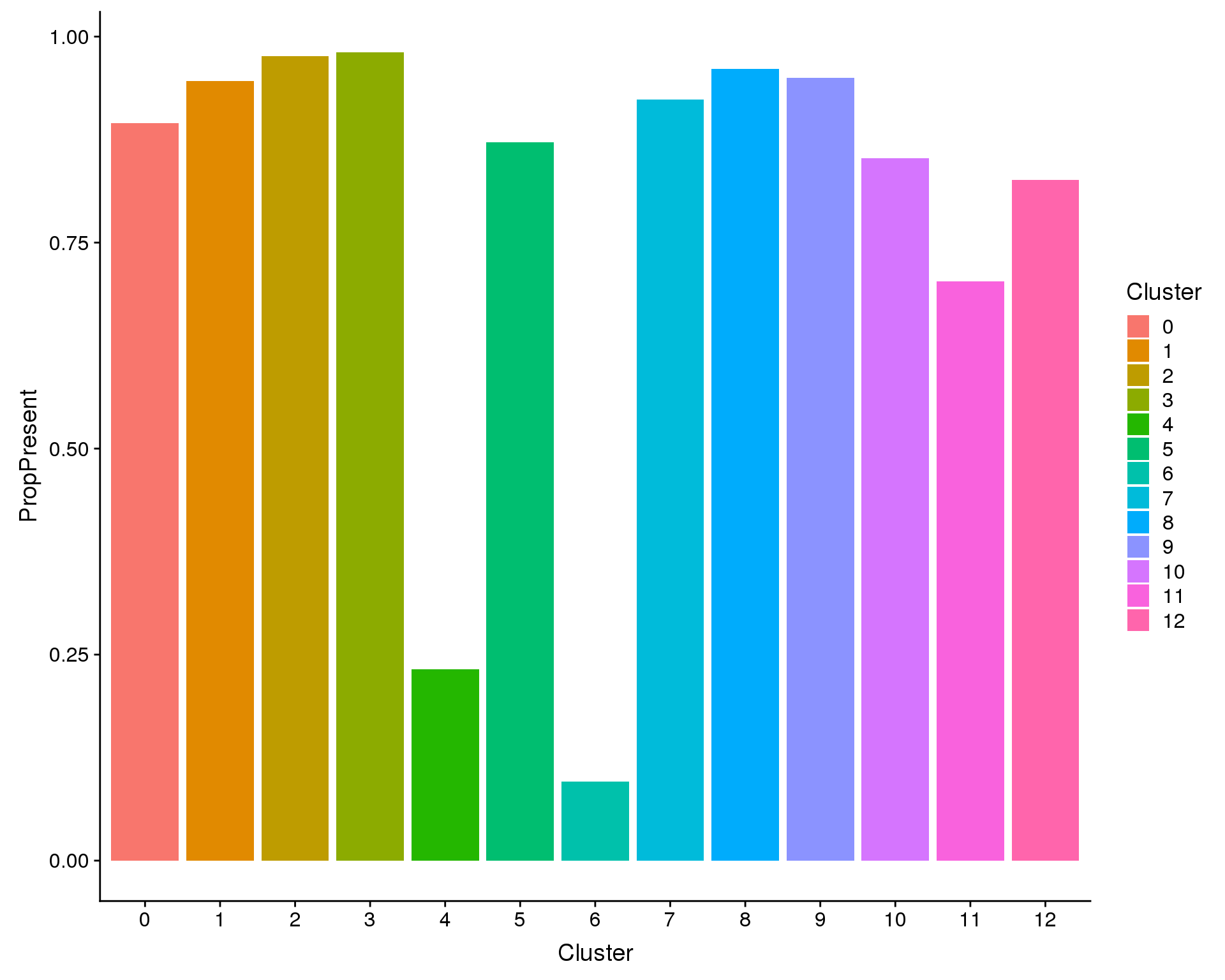
Expand here to see past versions of comp-present-1.png:
| Version | Author | Date |
|---|---|---|
| b8ba005 | Luke Zappia | 2019-02-24 |
Perhaps more importantly is how the cells that are present match up with the clusters we described previously. We can do this by making a heatmap of the Jaccard Index which measures the overlap between two sets (in this case of cells).
plot_data <- summariseClusts(cell_data, Cluster, PubCluster) %>%
    replace_na(list(Jaccard = 0))

ggplot(plot_data, aes(x = Cluster, y = PubCluster, fill = Jaccard)) +
    geom_tile() +
    scale_fill_viridis_c(limits = c(0, 1), name = "Jaccard\nindex") +
    coord_equal() +
    xlab("Cluster") +
    ylab("Published cluster") +
    theme_minimal() +
    theme(axis.text = element_text(size = 10, colour = "black"),
          axis.ticks = element_blank(),
          axis.title = element_text(size = 15),
          legend.key.height = unit(30, "pt"),
          legend.title = element_text(size = 15),
          legend.text = element_text(size = 10),
          panel.grid = element_blank())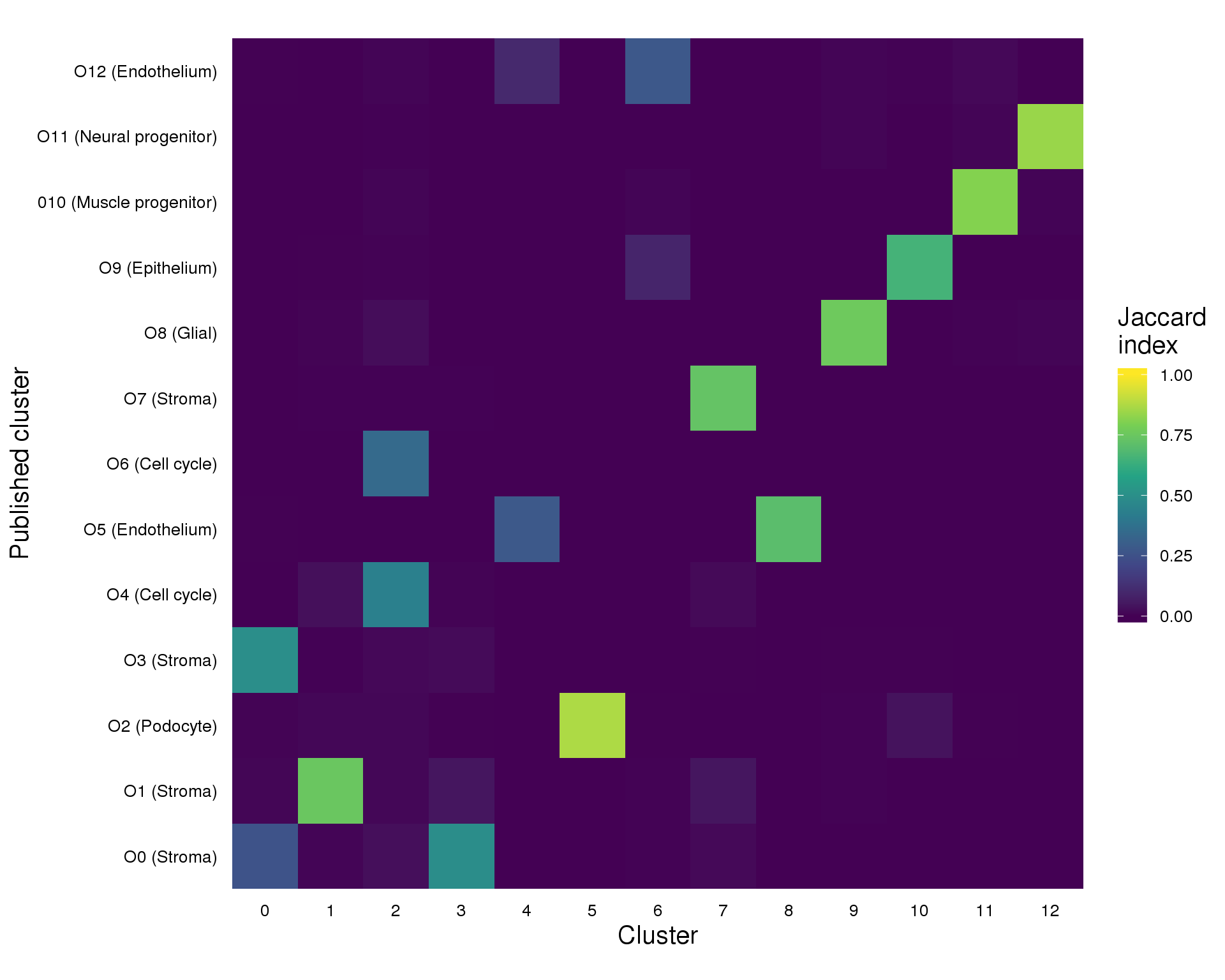
Expand here to see past versions of comp-jaccard-1.png:
| Version | Author | Date |
|---|---|---|
| b8ba005 | Luke Zappia | 2019-02-24 |
Figures
Gene selection
plot_data <- rowData(sce) %>%
    as.data.frame() %>%
    select(SeuratMean, SeuratDispScaled, SeuratSelected, M3DropAvgExpr,
           M3DropDropoutRate, M3DropDropoutExp, M3DropSelected, SelMethod)

plot_data_sel <- plot_data %>%
    filter(SelMethod != "False")

seurat_plot <- ggplot(plot_data,
       aes(x = SeuratMean, y = SeuratDispScaled, colour = SeuratSelected)) +
    geom_point(alpha = 0.3) +
    geom_vline(xintercept = x_low,  colour = "#7A52C7") +
    annotate("text", x = x_low, y = Inf, colour = "#7A52C7",
             label = x_low, angle = 90, hjust = 1, vjust = -1) +
    geom_vline(xintercept = x_high, colour = "#7A52C7") +
    annotate("text", x = x_high, y = Inf, colour = "#7A52C7",
             label = x_high, angle = 90, hjust = 1, vjust = -1) +
    geom_hline(yintercept = y_low,  colour = "#7A52C7") +
    annotate("text", x = Inf, y = y_low, colour = "#7A52C7",
             label = y_low, hjust = 1, vjust = -1) +
    scale_colour_manual(values = c("grey50", "#00ADEF"), name = "Selected") +
    annotate("text", x = x_low + 0.5 * (x_high - x_low), y = 10,
             colour = "#00ADEF", size = 5,
             label = paste(sum(plot_data$SeuratSelected), "selected")) +
    ggtitle("Seurat gene selection") +
    xlab("Gene mean (log)") +
    ylab("Seurat gene dispersion (scaled)") +
    theme_minimal() +
    theme(legend.position = "bottom")

m3drop_plot <- ggplot(plot_data,
       aes(x = M3DropAvgExpr, y = M3DropDropoutRate, colour = M3DropSelected)) +
    geom_point(alpha = 0.3) +
    geom_line(aes(y = M3DropDropoutExp), colour = "#7A52C7", size = 1) +
    annotate("text", x = 2, y = 0.9, colour = "#EC008C", size = 5,
             label = paste(sum(plot_data$M3DropSelected), "selected")) +
    scale_colour_manual(values = c("grey50", "#EC008C"), name = "Selected") +
    ggtitle("M3Drop gene selection") +
    xlab("M3Drop average expression") +
    ylab("M3Drop dropout rate") +
    theme_minimal() +
    theme(legend.position = "bottom")

comp_plot <- ggplot(plot_data, aes(x = SeuratDispScaled, y = M3DropDropoutRate)) +
    geom_point(alpha = 0.3, colour = "grey") +
    geom_point(data = plot_data_sel, aes(colour = SelMethod), alpha = 0.3) +
    scale_colour_manual(values = c("#8DC63F", "#EC008C", "#00ADEF")) +
    ggtitle("Comparison of gene selection methods") +
    xlab("Seurat gene dispersion (scaled)") +
    ylab("M3Drop dropout rate") +
    theme_minimal() +
    theme(legend.position = "bottom")

overlap_plot <- ggplot(plot_data_sel, aes(x = SelMethod, fill = SelMethod)) +
    geom_bar() +
    scale_fill_manual(values = c("#8DC63F", "#EC008C", "#00ADEF")) +
    coord_flip() +
    ggtitle("Overlap of selected genes") +
    ylab("Number of genes") +
    theme_minimal() +
    theme(legend.position = "none",
          axis.title.y = element_blank())

fig <- plot_grid(seurat_plot, m3drop_plot, comp_plot, overlap_plot, nrow = 2,
                 labels = "AUTO")

ggsave(here::here("output", DOCNAME, "gene-selection.pdf"), fig,
       width = 10, height = 8, scale = 1.2)
ggsave(here::here("output", DOCNAME, "gene-selection.png"), fig,
       width = 10, height = 8, scale = 1.2)

fig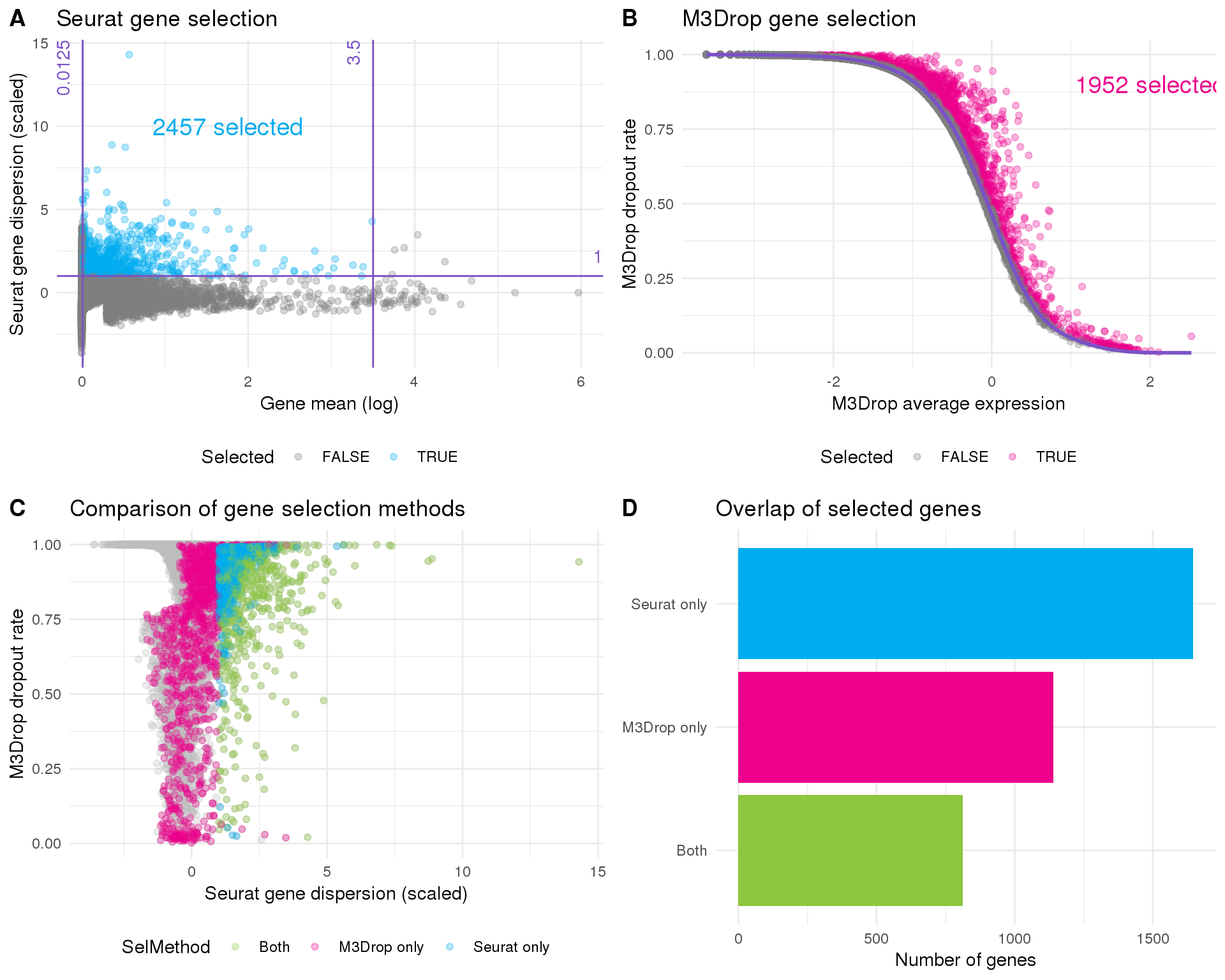
Resolution
res_y <- 10 - res / 0.1

ct_plot <- clustree(seurat, show_axis = TRUE) +
    annotate("rect",
             xmin = -11.8, xmax = 8, ymin = res_y - 0.4, ymax = res_y + 0.6,
             fill = alpha("grey", 0), colour = "#EC008C", size = 1) +
    ylab("Resolution") +
    theme(legend.position = "none",
          axis.text.y = element_text(),
          axis.title = element_text(),
          axis.title.x = element_blank(),
          panel.grid.major.y = element_line(colour = "grey92"))

gene_list <- c("TAGLN", "MAB21L2", "NPHS2", "PECAM1", "TTYH1", "STMN2",
               "PAX2", "MYOG")

plot_list <- lapply(gene_list, function(gene) {
    clustree(seurat, node_colour = gene, node_colour_aggr = "mean",
             exprs = "scale.data", node_size_range = c(2, 6),
             edge_width = 0.5, node_text_size = 0) +
        scale_colour_viridis_c(option = "plasma", begin = 0.3) +
        ggtitle(gene) +
        theme(legend.position = "none",
              plot.title = element_text(size = rel(1.2), hjust = 0.5,
                                        vjust = 1, margin = margin(5.5)))
})

genes_plot <- plot_grid(plotlist = plot_list, nrow = 2)

fig <- plot_grid(ct_plot, genes_plot, nrow = 2, labels = "AUTO")

ggsave(here::here("output", DOCNAME, "resolution-selection.pdf"), fig,
       width = 8, height = 8, scale = 1.3)
ggsave(here::here("output", DOCNAME, "resolution-selection.png"), fig,
       width = 8, height = 8, scale = 1.3)

fig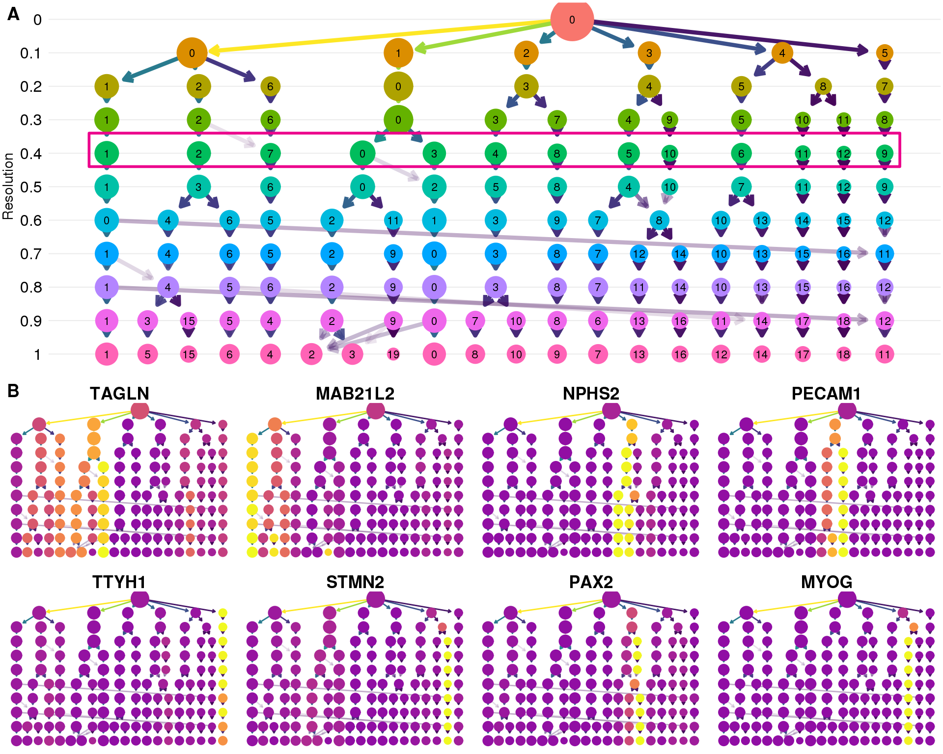
Validation
plot_data <- reducedDim(sce, "SeuratUMAP") %>%
    as.data.frame() %>%
    rename(UMAP1 = V1, UMAP2 = V2) %>%
    mutate(Cluster = colData(sce)$Cluster)

label_data <- plot_data %>%
    group_by(Cluster) %>%
    summarise(UMAP1 = mean(UMAP1),
              UMAP2 = mean(UMAP2))

umap_plot <- ggplot(plot_data, aes(x = UMAP1, y = UMAP2, colour = Cluster)) +
    geom_point(alpha = 0.3) +
    geom_point(data = label_data, shape = 21, size = 6, stroke = 1,
               fill = "white") +
    geom_text(data = label_data, aes(label = Cluster)) +
    ggtitle("Clusters in UMAP space") +
    theme_minimal() +
    theme(legend.position = "none")

sizes_plot <- ggplot(cell_data, aes(x = Cluster, fill = Cluster)) +
    geom_bar() +
    scale_y_continuous(breaks = seq(0, 1500, 200)) +
    ggtitle("Cluster sizes") +
    ylab("Number of cells") +
    theme_minimal() +
    theme(legend.position = "none",
          axis.title.x = element_blank())

plot_data <- cell_data %>%
    group_by(Cluster, SelMethod) %>%
    summarise(Count = n()) %>%
    mutate(Prop = Count / sum(Count)) %>%
    mutate(SelMethod = factor(
        SelMethod,
        levels = c("Both", "CellRanger", "emptyDrops"),
        labels = c("Both", "Cell Ranger v3 only", "EmptyDrops only")
    ))

sel_plot <- ggplot(plot_data, aes(x = Cluster, y = Prop, fill = SelMethod)) +
    geom_col() +
    scale_fill_manual(values = c("#EC008C", "#00ADEF", "#8DC63F")) +
    ggtitle("Selection method by cluster") +
    ylab("Proportion of cluster") +
    theme_minimal() +
    theme(legend.position = "bottom",
          axis.title.x = element_blank(),
          legend.title = element_blank())

plot_data <- cell_data %>%
    group_by(Cluster, CellCycle) %>%
    summarise(Count = n()) %>%
    mutate(Prop = Count / sum(Count))

cycle_plot <- ggplot(plot_data, aes(x = Cluster, y = Prop, fill = CellCycle)) +
    geom_col() +
    scale_fill_manual(values = c("#EC008C", "#00ADEF", "#8DC63F")) +
    ggtitle("Cell cycle phase by cluster") +
    ylab("Proportion of cluster") +
    theme_minimal() +
    theme(legend.position = "bottom",
          axis.title.x = element_blank(),
          legend.title = element_blank())

counts_plot <- ggplot(cell_data, aes(x = Cluster, y = log10_total_counts)) +
    geom_sina(aes(colour = Cluster), size = 0.5) +
    ggtitle("Total counts by cluster") +
    ylab(expression("Total counts ("*log["10"]*")")) +
    theme_minimal() +
    theme(legend.position = "none",
          axis.title.x = element_blank())

mt_plot <- ggplot(cell_data, aes(x = Cluster, y = pct_counts_MT)) +
    geom_sina(aes(colour = Cluster), size = 0.5) +
    ggtitle("Mitochondrial counts by cluster") +
    ylab("% counts mitochondrial") +
    theme_minimal() +
    theme(legend.position = "none",
          axis.title.x = element_blank())

fig <- plot_grid(umap_plot, sizes_plot, sel_plot, cycle_plot, counts_plot,
                 mt_plot, ncol = 2, labels = "AUTO")

ggsave(here::here("output", DOCNAME, "cluster-validation.pdf"), fig,
       width = 7, height = 10, scale = 1.2)
ggsave(here::here("output", DOCNAME, "cluster-validation.png"), fig,
       width = 7, height = 10, scale = 1.2)

fig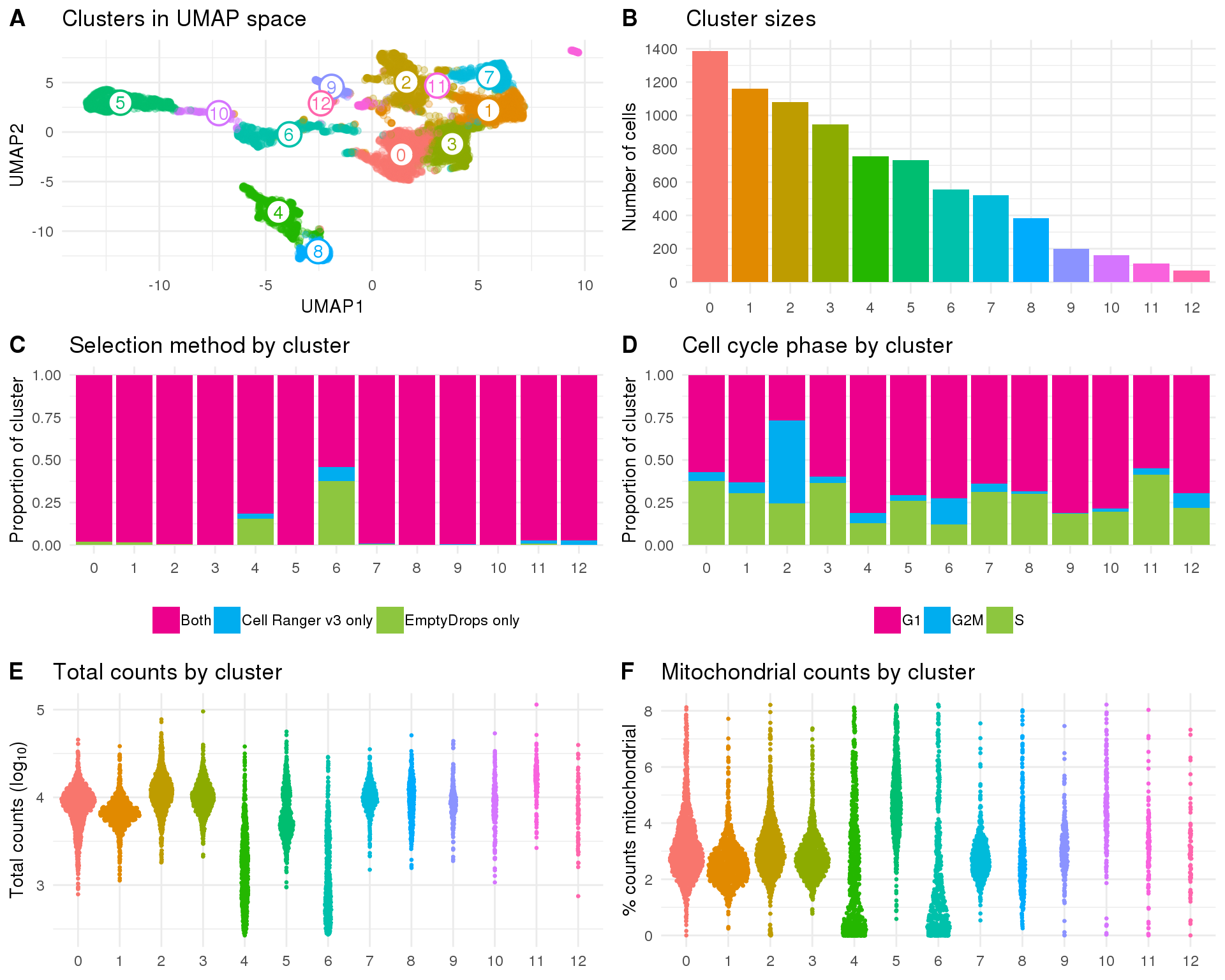
Comparison
plot_data <- cell_data %>%
    mutate(Present = !is.na(PubCluster)) %>%
    group_by(Cluster) %>%
    summarise(PropPresent = sum(Present) / n())

present_plot <- ggplot(plot_data,
                       aes(x = Cluster, y = PropPresent, fill = Cluster)) +
    geom_col() +
    ggtitle("Presence in published analysis") +
    ylab("Proportion of cluster") +
    theme_minimal() +
    theme(legend.position = "none",
          axis.title.x = element_blank())

plot_data <- summariseClusts(cell_data, Cluster, PubCluster) %>%
    replace_na(list(Jaccard = 0))

overlap_plot <- ggplot(plot_data,
                       aes(x = Cluster, y = PubCluster, fill = Jaccard)) +
    geom_tile() +
    scale_fill_viridis_c(limits = c(0, 1), name = "Jaccard\nindex") +
    coord_equal() +
    ggtitle("Overlap with published clusters") +
    xlab("Cluster") +
    ylab("Published cluster") +
    theme_minimal() +
    theme(plot.title = element_text(size = rel(1.2), hjust = -0.65, vjust = 1.5,
                                    margin = margin(1)),
          axis.text = element_text(size = 9, colour = "black"),
          axis.ticks = element_blank(),
          axis.title = element_text(size = 12),
          legend.key.height = unit(30, "pt"),
          legend.title = element_text(size = 12),
          legend.text = element_text(size = 9),
          panel.grid = element_blank())

fig <- plot_grid(present_plot, overlap_plot, ncol = 1,
                 rel_heights = c(0.5, 1), labels = "AUTO")

ggsave(here::here("output", DOCNAME, "cluster-comparison.pdf"), fig,
       width = 7, height = 7.5, scale = 1)
ggsave(here::here("output", DOCNAME, "cluster-comparison.png"), fig,
       width = 7, height = 7.5, scale = 1)

fig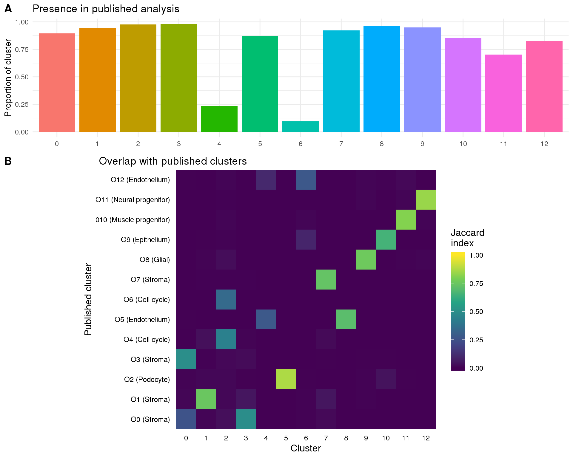
Summary
We performed graph based clustering using Seurat and identified 13 clusters.
Parameters
This table describes parameters used and set in this document.
params <- list(
    list(
        Parameter = "seurat_thresh",
        Value = c(exp_low = x_low, exp_high = x_high, disp_low = y_low,
                  disp_high = y_high),
        Description = paste("Seurat selection thresholds",
                            "(low expression, high expression,",
                            "low dispersion, high dispersion)")
    ),
    list(
        Parameter = "sel_seurat",
        Value = sum(rowData(sce)$SeuratSelected),
        Description = "Number of genes selected by the Seurat method"
    ),
    list(
        Parameter = "m3drop_thresh",
        Value = m3drop_q,
        Description = "M3Drop q-value threshold"
    ),
    list(
        Parameter = "sel_m3drop",
        Value = sum(rowData(sce)$M3DropSelected),
        Description = "Number of genes selected by the M3Drop method"
    ),
    list(
        Parameter = "sel_genes",
        Value = length(seurat@var.genes),
        Description = "Number of selected genes"
    ),
    list(
        Parameter = "n_pcs",
        Value = n_pcs,
        Description = "Selected number of principal components for clustering"
    ),
    list(
        Parameter = "knn",
        Value = knn,
        Description = "Number of neighbours for SNN graph"
    ),
    list(
        Parameter = "resolutions",
        Value = resolutions,
        Description = "Range of possible clustering resolutions"
    ),
    list(
        Parameter = "res",
        Value = res,
        Description = "Selected resolution parameter for clustering"
    ),
    list(
        Parameter = "n_clusts",
        Value = n_clusts,
        Description = "Number of clusters produced by selected resolution"
    )
)

params <- jsonlite::toJSON(params, pretty = TRUE)
knitr::kable(jsonlite::fromJSON(params))| Parameter | Value | Description |
|---|---|---|
| seurat_thresh | c(0.0125, 3.5, 1, Inf) | Seurat selection thresholds (low expression, high expression, low dispersion, high dispersion) |
| sel_seurat | 2457 | Number of genes selected by the Seurat method |
| m3drop_thresh | 0.01 | M3Drop q-value threshold |
| sel_m3drop | 1952 | Number of genes selected by the M3Drop method |
| sel_genes | 1952 | Number of selected genes |
| n_pcs | 15 | Selected number of principal components for clustering |
| knn | 30 | Number of neighbours for SNN graph |
| resolutions | c(0, 0.1, 0.2, 0.3, 0.4, 0.5, 0.6, 0.7, 0.8, 0.9, 1) | Range of possible clustering resolutions |
| res | 0.4 | Selected resolution parameter for clustering |
| n_clusts | 13 | Number of clusters produced by selected resolution |
Output files
This table describes the output files produced by this document. Right click and Save Link As… to download the results.
write_rds(sce, here::here("data/processed/03-clustered.Rds"))
write_rds(seurat, here::here("data/processed/03-seurat.Rds"))
counts_sel <- as.matrix(counts(sce)[sel_genes$Name, ])
sce_sel <- SingleCellExperiment(assays = list(counts = counts_sel),
colData = colData(sce))
scle_sel <- LoomExperiment(sce_sel)
loom_path <- here::here("data/processed/03-clustered-sel.loom")
if (file.exists(loom_path)) {
file.remove(loom_path)
}[1] TRUEexport(scle_sel, loom_path)avg_expr <- AverageExpression(seurat, show.progress = FALSE) %>%
rename_all(function(x) {paste0("MeanC", x)}) %>%
rownames_to_column("Gene")
prop_expr <- AverageDetectionRate(seurat) %>%
rename_all(function(x) {paste0("PropC", x)}) %>%
rownames_to_column("Gene")
alt_cols <- c(rbind(colnames(prop_expr), colnames(avg_expr)))[-1]
cluster_expr <- avg_expr %>%
left_join(prop_expr, by = "Gene") %>%
select(alt_cols)
cluster_assign <- colData(sce) %>%
as.data.frame() %>%
select(Cell, Dataset, Sample, Barcode, Cluster)dir.create(here::here("output", DOCNAME), showWarnings = FALSE)
readr::write_lines(params, here::here("output", DOCNAME, "parameters.json"))
writeGeneTable(sel_genes, here::here("output", DOCNAME, "selected_genes.csv"))
readr::write_tsv(cluster_assign,
here::here("output", DOCNAME, "cluster_assignments.tsv.gz"))
readr::write_tsv(cluster_expr,
here::here("output", DOCNAME, "cluster_expression.tsv.gz"))
knitr::kable(data.frame(
File = c(
getDownloadLink("parameters.json", DOCNAME),
getDownloadLink("selected_genes.csv.zip", DOCNAME),
getDownloadLink("cluster_assignments.tsv.gz", DOCNAME),
getDownloadLink("cluster_expression.tsv.gz", DOCNAME),
getDownloadLink("gene-selection.png", DOCNAME),
getDownloadLink("gene-selection.pdf", DOCNAME),
getDownloadLink("resolution-selection.png", DOCNAME),
getDownloadLink("resolution-selection.pdf", DOCNAME),
getDownloadLink("cluster-validation.png", DOCNAME),
getDownloadLink("cluster-validation.pdf", DOCNAME),
getDownloadLink("cluster-comparison.png", DOCNAME),
getDownloadLink("cluster-comparison.pdf", DOCNAME)
),
Description = c(
"Parameters set and used in this analysis",
"Selected genes (zipped CSV)",
"Cluster assignments for each cell (gzipped TSV)",
"Cluster expression for each gene (gzipped TSV)",
"Gene selection figure (PNG)",
"Gene selection figure (PDF)",
"Resolution selection figure (PNG)",
"Resolution selection figure (PDF)",
"Cluster validation figure (PNG)",
"Cluster validation figure (PDF)",
"Cluster comparison figure (PNG)",
"Cluster comparison figure (PDF)"
)
))| File | Description |
|---|---|
| parameters.json | Parameters set and used in this analysis |
| selected_genes.csv.zip | Selected genes (zipped CSV) |
| cluster_assignments.tsv.gz | Cluster assignments for each cell (gzipped TSV) |
| cluster_expression.tsv.gz | Cluster expression for each gene (gzipped TSV) |
| gene-selection.png | Gene selection figure (PNG) |
| gene-selection.pdf | Gene selection figure (PDF) |
| resolution-selection.png | Resolution selection figure (PNG) |
| resolution-selection.pdf | Resolution selection figure (PDF) |
| cluster-validation.png | Cluster validation figure (PNG) |
| cluster-validation.pdf | Cluster validation figure (PDF) |
| cluster-comparison.png | Cluster comparison figure (PNG) |
| cluster-comparison.pdf | Cluster comparison figure (PDF) |
Session information
devtools::session_info()─ Session info ──────────────────────────────────────────────────────────
setting value
version R version 3.5.0 (2018-04-23)
os CentOS release 6.7 (Final)
system x86_64, linux-gnu
ui X11
language (EN)
collate en_US.UTF-8
ctype en_US.UTF-8
tz Australia/Melbourne
date 2019-04-03
─ Packages ──────────────────────────────────────────────────────────────
! package * version date lib
acepack 1.4.1 2016-10-29 [1]
ape 5.2 2018-09-24 [1]
assertthat 0.2.0 2017-04-11 [1]
backports 1.1.3 2018-12-14 [1]
base64enc 0.1-3 2015-07-28 [1]
bbmle 1.0.20 2017-10-30 [1]
beeswarm 0.2.3 2016-04-25 [1]
bibtex 0.4.2 2017-06-30 [1]
bindr 0.1.1 2018-03-13 [1]
bindrcpp 0.2.2 2018-03-29 [1]
Biobase * 2.42.0 2018-10-30 [1]
BiocGenerics * 0.28.0 2018-10-30 [1]
BiocParallel * 1.16.5 2019-01-04 [1]
Biostrings 2.50.2 2019-01-03 [1]
bit 1.1-14 2018-05-29 [1]
bit64 0.9-7 2017-05-08 [1]
bitops 1.0-6 2013-08-17 [1]
broom 0.5.1 2018-12-05 [1]
callr 3.1.1 2018-12-21 [1]
caTools 1.17.1.1 2018-07-20 [1]
cellranger 1.1.0 2016-07-27 [1]
checkmate 1.9.1 2019-01-15 [1]
P class 7.3-14 2015-08-30 [5]
cli 1.0.1 2018-09-25 [1]
P cluster 2.0.7-1 2018-04-13 [5]
clustree * 0.3.0 2019-02-24 [1]
P codetools 0.2-15 2016-10-05 [5]
colorspace 1.4-0 2019-01-13 [1]
cowplot * 0.9.4 2019-01-08 [1]
crayon 1.3.4 2017-09-16 [1]
data.table 1.12.0 2019-01-13 [1]
DelayedArray * 0.8.0 2018-10-30 [1]
DelayedMatrixStats 1.4.0 2018-10-30 [1]
DEoptimR 1.0-8 2016-11-19 [1]
desc 1.2.0 2018-05-01 [1]
devtools 2.0.1 2018-10-26 [1]
digest 0.6.18 2018-10-10 [1]
diptest 0.75-7 2016-12-05 [1]
doSNOW 1.0.16 2017-12-13 [1]
dplyr * 0.7.8 2018-11-10 [1]
dtw 1.20-1 2018-05-18 [1]
evaluate 0.12 2018-10-09 [1]
farver 1.1.0 2018-11-20 [1]
fitdistrplus 1.0-14 2019-01-23 [1]
flexmix 2.3-14 2017-04-28 [1]
forcats * 0.3.0 2018-02-19 [1]
foreach 1.4.4 2017-12-12 [1]
P foreign 0.8-71 2018-07-20 [5]
Formula 1.2-3 2018-05-03 [1]
fpc 2.1-11.1 2018-07-20 [1]
fs 1.2.6 2018-08-23 [1]
gbRd 0.4-11 2012-10-01 [1]
gdata 2.18.0 2017-06-06 [1]
generics 0.0.2 2018-11-29 [1]
GenomeInfoDb * 1.18.1 2018-11-12 [1]
GenomeInfoDbData 1.2.0 2019-01-15 [1]
GenomicAlignments 1.18.1 2019-01-04 [1]
GenomicRanges * 1.34.0 2018-10-30 [1]
ggbeeswarm 0.6.0 2017-08-07 [1]
ggforce * 0.1.3 2018-07-07 [1]
ggplot2 * 3.1.0 2018-10-25 [1]
ggraph * 1.0.2 2018-07-07 [1]
ggrepel 0.8.0 2018-05-09 [1]
ggridges 0.5.1 2018-09-27 [1]
git2r 0.24.0 2019-01-07 [1]
glue 1.3.0 2018-07-17 [1]
gplots 3.0.1.1 2019-01-27 [1]
gridExtra 2.3 2017-09-09 [1]
gtable 0.2.0 2016-02-26 [1]
gtools 3.8.1 2018-06-26 [1]
haven 2.0.0 2018-11-22 [1]
HDF5Array 1.10.1 2018-12-05 [1]
hdf5r 1.0.1 2018-10-07 [1]
here 0.1 2017-05-28 [1]
Hmisc 4.2-0 2019-01-26 [1]
hms 0.4.2 2018-03-10 [1]
htmlTable 1.13.1 2019-01-07 [1]
htmltools 0.3.6 2017-04-28 [1]
htmlwidgets 1.3 2018-09-30 [1]
httr 1.4.0 2018-12-11 [1]
ica 1.0-2 2018-05-24 [1]
igraph 1.2.2 2018-07-27 [1]
IRanges * 2.16.0 2018-10-30 [1]
irlba 2.3.3 2019-02-05 [1]
iterators 1.0.10 2018-07-13 [1]
jsonlite 1.6 2018-12-07 [1]
kernlab 0.9-27 2018-08-10 [1]
P KernSmooth 2.23-15 2015-06-29 [5]
knitr * 1.21 2018-12-10 [1]
lars 1.2 2013-04-24 [1]
P lattice 0.20-35 2017-03-25 [5]
latticeExtra 0.6-28 2016-02-09 [1]
lazyeval 0.2.1 2017-10-29 [1]
lmtest 0.9-36 2018-04-04 [1]
LoomExperiment * 1.0.2 2019-01-04 [1]
lsei 1.2-0 2017-10-23 [1]
lubridate 1.7.4 2018-04-11 [1]
M3Drop * 3.10.3 2019-01-23 [1]
magrittr 1.5 2014-11-22 [1]
P MASS 7.3-50 2018-04-30 [5]
P Matrix * 1.2-14 2018-04-09 [5]
matrixStats * 0.54.0 2018-07-23 [1]
mclust 5.4.2 2018-11-17 [1]
memoise 1.1.0 2017-04-21 [1]
metap 1.1 2019-02-06 [1]
P mgcv 1.8-24 2018-06-18 [5]
mixtools 1.1.0 2017-03-10 [1]
modelr 0.1.3 2019-02-05 [1]
modeltools 0.2-22 2018-07-16 [1]
munsell 0.5.0 2018-06-12 [1]
mvtnorm 1.0-8 2018-05-31 [1]
P nlme 3.1-137 2018-04-07 [5]
P nnet 7.3-12 2016-02-02 [5]
npsurv 0.4-0 2017-10-14 [1]
numDeriv * 2016.8-1 2016-08-27 [1]
pbapply 1.4-0 2019-02-05 [1]
pillar 1.3.1 2018-12-15 [1]
pkgbuild 1.0.2 2018-10-16 [1]
pkgconfig 2.0.2 2018-08-16 [1]
pkgload 1.0.2 2018-10-29 [1]
plyr 1.8.4 2016-06-08 [1]
png 0.1-7 2013-12-03 [1]
prabclus 2.2-7 2019-01-17 [1]
prettyunits 1.0.2 2015-07-13 [1]
processx 3.2.1 2018-12-05 [1]
proxy 0.4-22 2018-04-08 [1]
ps 1.3.0 2018-12-21 [1]
purrr * 0.3.0 2019-01-27 [1]
R.methodsS3 1.7.1 2016-02-16 [1]
R.oo 1.22.0 2018-04-22 [1]
R.utils 2.7.0 2018-08-27 [1]
R6 2.3.0 2018-10-04 [1]
RANN 2.6.1 2019-01-08 [1]
RColorBrewer 1.1-2 2014-12-07 [1]
Rcpp 1.0.0 2018-11-07 [1]
RCurl 1.95-4.11 2018-07-15 [1]
Rdpack 0.10-1 2018-10-04 [1]
readr * 1.3.1 2018-12-21 [1]
readxl 1.2.0 2018-12-19 [1]
reldist 1.6-6 2016-10-09 [1]
remotes 2.0.2 2018-10-30 [1]
reshape2 1.4.3 2017-12-11 [1]
reticulate 1.10 2018-08-05 [1]
rhdf5 * 2.26.2 2019-01-02 [1]
Rhdf5lib 1.4.2 2018-12-03 [1]
rlang 0.3.1 2019-01-08 [1]
rmarkdown 1.11 2018-12-08 [1]
robustbase 0.93-3 2018-09-21 [1]
ROCR 1.0-7 2015-03-26 [1]
P rpart 4.1-13 2018-02-23 [5]
rprojroot 1.3-2 2018-01-03 [1]
Rsamtools 1.34.1 2019-01-31 [1]
rstudioapi 0.9.0 2019-01-09 [1]
rtracklayer * 1.42.1 2018-11-22 [1]
Rtsne 0.15 2018-11-10 [1]
rvest 0.3.2 2016-06-17 [1]
S4Vectors * 0.20.1 2018-11-09 [1]
scales 1.0.0 2018-08-09 [1]
scater * 1.10.1 2019-01-04 [1]
SDMTools 1.1-221 2014-08-05 [1]
segmented 0.5-3.0 2017-11-30 [1]
sessioninfo 1.1.1 2018-11-05 [1]
Seurat * 2.3.4 2018-07-20 [1]
SingleCellExperiment * 1.4.1 2019-01-04 [1]
snow 0.4-3 2018-09-14 [1]
statmod 1.4.30 2017-06-18 [1]
stringi 1.2.4 2018-07-20 [1]
stringr * 1.3.1 2018-05-10 [1]
SummarizedExperiment * 1.12.0 2018-10-30 [1]
P survival 2.42-6 2018-07-13 [5]
testthat 2.0.1 2018-10-13 [4]
tibble * 2.0.1 2019-01-12 [1]
tidyr * 0.8.2 2018-10-28 [1]
tidyselect 0.2.5 2018-10-11 [1]
tidyverse * 1.2.1 2017-11-14 [1]
trimcluster 0.1-2.1 2018-07-20 [1]
tsne 0.1-3 2016-07-15 [1]
tweenr 1.0.1 2018-12-14 [1]
units 0.6-2 2018-12-05 [1]
usethis 1.4.0 2018-08-14 [1]
vipor 0.4.5 2017-03-22 [1]
viridis * 0.5.1 2018-03-29 [1]
viridisLite * 0.3.0 2018-02-01 [1]
whisker 0.3-2 2013-04-28 [1]
withr 2.1.2 2018-03-15 [1]
workflowr 1.1.1 2018-07-06 [1]
xfun 0.4 2018-10-23 [1]
XML 3.98-1.16 2018-08-19 [1]
xml2 1.2.0 2018-01-24 [1]
XVector 0.22.0 2018-10-30 [1]
yaml 2.2.0 2018-07-25 [1]
zlibbioc 1.28.0 2018-10-30 [1]
zoo 1.8-4 2018-09-19 [1]
source
CRAN (R 3.5.0)
CRAN (R 3.5.0)
CRAN (R 3.5.0)
CRAN (R 3.5.0)
CRAN (R 3.5.0)
CRAN (R 3.5.0)
CRAN (R 3.5.0)
CRAN (R 3.5.0)
CRAN (R 3.5.0)
CRAN (R 3.5.0)
Bioconductor
Bioconductor
Bioconductor
Bioconductor
CRAN (R 3.5.0)
CRAN (R 3.5.0)
CRAN (R 3.5.0)
CRAN (R 3.5.0)
CRAN (R 3.5.0)
CRAN (R 3.5.0)
CRAN (R 3.5.0)
CRAN (R 3.5.0)
CRAN (R 3.5.0)
CRAN (R 3.5.0)
CRAN (R 3.5.0)
CRAN (R 3.5.0)
CRAN (R 3.5.0)
CRAN (R 3.5.0)
CRAN (R 3.5.0)
CRAN (R 3.5.0)
CRAN (R 3.5.0)
Bioconductor
Bioconductor
CRAN (R 3.5.0)
CRAN (R 3.5.0)
CRAN (R 3.5.0)
CRAN (R 3.5.0)
CRAN (R 3.5.0)
CRAN (R 3.5.0)
CRAN (R 3.5.0)
CRAN (R 3.5.0)
CRAN (R 3.5.0)
CRAN (R 3.5.0)
CRAN (R 3.5.0)
CRAN (R 3.5.0)
CRAN (R 3.5.0)
CRAN (R 3.5.0)
CRAN (R 3.5.0)
CRAN (R 3.5.0)
CRAN (R 3.5.0)
CRAN (R 3.5.0)
CRAN (R 3.5.0)
CRAN (R 3.5.0)
CRAN (R 3.5.0)
Bioconductor
Bioconductor
Bioconductor
Bioconductor
CRAN (R 3.5.0)
CRAN (R 3.5.0)
CRAN (R 3.5.0)
CRAN (R 3.5.0)
CRAN (R 3.5.0)
CRAN (R 3.5.0)
CRAN (R 3.5.0)
CRAN (R 3.5.0)
CRAN (R 3.5.0)
CRAN (R 3.5.0)
CRAN (R 3.5.0)
CRAN (R 3.5.0)
CRAN (R 3.5.0)
Bioconductor
CRAN (R 3.5.0)
CRAN (R 3.5.0)
CRAN (R 3.5.0)
CRAN (R 3.5.0)
CRAN (R 3.5.0)
CRAN (R 3.5.0)
CRAN (R 3.5.0)
CRAN (R 3.5.0)
CRAN (R 3.5.0)
CRAN (R 3.5.0)
Bioconductor
CRAN (R 3.5.0)
CRAN (R 3.5.0)
CRAN (R 3.5.0)
CRAN (R 3.5.0)
CRAN (R 3.5.0)
CRAN (R 3.5.0)
CRAN (R 3.5.0)
CRAN (R 3.5.0)
CRAN (R 3.5.0)
CRAN (R 3.5.0)
CRAN (R 3.5.0)
Bioconductor
CRAN (R 3.5.0)
CRAN (R 3.5.0)
Github (tallulandrews/M3Drop@d825b91)
CRAN (R 3.5.0)
CRAN (R 3.5.0)
CRAN (R 3.5.0)
CRAN (R 3.5.0)
CRAN (R 3.5.0)
CRAN (R 3.5.0)
CRAN (R 3.5.0)
CRAN (R 3.5.0)
CRAN (R 3.5.0)
CRAN (R 3.5.0)
CRAN (R 3.5.0)
CRAN (R 3.5.0)
CRAN (R 3.5.0)
CRAN (R 3.5.0)
CRAN (R 3.5.0)
CRAN (R 3.5.0)
CRAN (R 3.5.0)
CRAN (R 3.5.0)
CRAN (R 3.5.0)
CRAN (R 3.5.0)
CRAN (R 3.5.0)
CRAN (R 3.5.0)
CRAN (R 3.5.0)
CRAN (R 3.5.0)
CRAN (R 3.5.0)
CRAN (R 3.5.0)
CRAN (R 3.5.0)
CRAN (R 3.5.0)
CRAN (R 3.5.0)
CRAN (R 3.5.0)
CRAN (R 3.5.0)
CRAN (R 3.5.0)
CRAN (R 3.5.0)
CRAN (R 3.5.0)
CRAN (R 3.5.0)
CRAN (R 3.5.0)
CRAN (R 3.5.0)
CRAN (R 3.5.0)
CRAN (R 3.5.0)
CRAN (R 3.5.0)
CRAN (R 3.5.0)
CRAN (R 3.5.0)
CRAN (R 3.5.0)
CRAN (R 3.5.0)
CRAN (R 3.5.0)
Bioconductor
Bioconductor
CRAN (R 3.5.0)
CRAN (R 3.5.0)
CRAN (R 3.5.0)
CRAN (R 3.5.0)
CRAN (R 3.5.0)
CRAN (R 3.5.0)
Bioconductor
CRAN (R 3.5.0)
Bioconductor
CRAN (R 3.5.0)
CRAN (R 3.5.0)
Bioconductor
CRAN (R 3.5.0)
Bioconductor
CRAN (R 3.5.0)
CRAN (R 3.5.0)
CRAN (R 3.5.0)
CRAN (R 3.5.0)
Bioconductor
CRAN (R 3.5.0)
CRAN (R 3.5.0)
CRAN (R 3.5.0)
CRAN (R 3.5.0)
Bioconductor
CRAN (R 3.5.0)
CRAN (R 3.5.0)
CRAN (R 3.5.0)
CRAN (R 3.5.0)
CRAN (R 3.5.0)
CRAN (R 3.5.0)
CRAN (R 3.5.0)
CRAN (R 3.5.0)
CRAN (R 3.5.0)
CRAN (R 3.5.0)
CRAN (R 3.5.0)
CRAN (R 3.5.0)
CRAN (R 3.5.0)
CRAN (R 3.5.0)
CRAN (R 3.5.0)
CRAN (R 3.5.0)
CRAN (R 3.5.0)
CRAN (R 3.5.0)
CRAN (R 3.5.0)
CRAN (R 3.5.0)
Bioconductor
CRAN (R 3.5.0)
Bioconductor
CRAN (R 3.5.0)
[1] /group/bioi1/luke/analysis/phd-thesis-analysis/packrat/lib/x86_64-pc-linux-gnu/3.5.0
[2] /group/bioi1/luke/analysis/phd-thesis-analysis/packrat/lib-ext/x86_64-pc-linux-gnu/3.5.0
[3] /group/bioi1/luke/analysis/phd-thesis-analysis/packrat/lib-R/x86_64-pc-linux-gnu/3.5.0
[4] /home/luke.zappia/R/x86_64-pc-linux-gnu-library/3.5
[5] /usr/local/installed/R/3.5.0/lib64/R/library
P ── Loaded and on-disk path mismatch.This reproducible R Markdown analysis was created with workflowr 1.1.1