Marker genes
Last updated: 2019-04-03
workflowr checks: (Click a bullet for more information)-
✔ R Markdown file: up-to-date
Great! Since the R Markdown file has been committed to the Git repository, you know the exact version of the code that produced these results.
-
✔ Environment: empty
Great job! The global environment was empty. Objects defined in the global environment can affect the analysis in your R Markdown file in unknown ways. For reproduciblity it’s best to always run the code in an empty environment.
-
✔ Seed:
set.seed(20190110)The command
set.seed(20190110)was run prior to running the code in the R Markdown file. Setting a seed ensures that any results that rely on randomness, e.g. subsampling or permutations, are reproducible. -
✔ Session information: recorded
Great job! Recording the operating system, R version, and package versions is critical for reproducibility.
-
Great! You are using Git for version control. Tracking code development and connecting the code version to the results is critical for reproducibility. The version displayed above was the version of the Git repository at the time these results were generated.✔ Repository version: 5870e6e
Note that you need to be careful to ensure that all relevant files for the analysis have been committed to Git prior to generating the results (you can usewflow_publishorwflow_git_commit). workflowr only checks the R Markdown file, but you know if there are other scripts or data files that it depends on. Below is the status of the Git repository when the results were generated:
Note that any generated files, e.g. HTML, png, CSS, etc., are not included in this status report because it is ok for generated content to have uncommitted changes.Ignored files: Ignored: .DS_Store Ignored: .Rhistory Ignored: .Rproj.user/ Ignored: ._.DS_Store Ignored: analysis/cache/ Ignored: build-logs/ Ignored: data/alevin/ Ignored: data/cellranger/ Ignored: data/processed/ Ignored: data/published/ Ignored: output/.DS_Store Ignored: output/._.DS_Store Ignored: output/03-clustering/selected_genes.csv.zip Ignored: output/04-marker-genes/de_genes.csv.zip Ignored: packrat/.DS_Store Ignored: packrat/._.DS_Store Ignored: packrat/lib-R/ Ignored: packrat/lib-ext/ Ignored: packrat/lib/ Ignored: packrat/src/ Untracked files: Untracked: DGEList.Rds Untracked: output/90-methods/package-versions.json Untracked: scripts/build.pbs Unstaged changes: Modified: analysis/_site.yml Modified: output/01-preprocessing/droplet-selection.pdf Modified: output/01-preprocessing/parameters.json Modified: output/01-preprocessing/selection-comparison.pdf Modified: output/01B-alevin/alevin-comparison.pdf Modified: output/01B-alevin/parameters.json Modified: output/02-quality-control/qc-thresholds.pdf Modified: output/02-quality-control/qc-validation.pdf Modified: output/03-clustering/cluster-comparison.pdf Modified: output/03-clustering/cluster-validation.pdf Modified: output/04-marker-genes/de-results.pdf
Expand here to see past versions:
| File | Version | Author | Date | Message |
|---|---|---|---|---|
| Rmd | 5870e6e | Luke Zappia | 2019-04-03 | Adjust figures and fix names |
| html | 33ac14f | Luke Zappia | 2019-03-20 | Tidy up website |
| html | ae75188 | Luke Zappia | 2019-03-06 | Revise figures after proofread |
| html | 2693e97 | Luke Zappia | 2019-03-05 | Add methods page |
| html | b610506 | Luke Zappia | 2019-02-27 | Add marker genes figure |
| html | 40b358f | Luke Zappia | 2019-02-13 | Assign clusters |
| html | 8f826ef | Luke Zappia | 2019-02-08 | Rebuild site and tidy |
| Rmd | fdf3fe8 | Luke Zappia | 2019-02-08 | Add marker gene testing |
# scRNA-seq
library("SingleCellExperiment")
library("scater")

# Differential expression
library("edgeR")

# Plotting
library("cowplot")

# Presentation
library("knitr")

# Tidyverse
library("tidyverse")
source(here::here("R/plotting.R"))
source(here::here("R/output.R"))clust_path <- here::here("data/processed/03-clustered.Rds")bpparam5 <- BiocParallel::MulticoreParam(workers = 5)
bpparam3 <- BiocParallel::MulticoreParam(workers = 3)Introduction
In this document we are going to identify marker genes for the clusters previously defined using Seurat using the edgeR package and use these genes to assign cell type labels to the clusters.
if (file.exists(clust_path)) {
    sce <- read_rds(clust_path)
} else {
    stop("Clustered dataset is missing. ",
         "Please run '03-clustering.Rmd' first.",
         call. = FALSE)
}

n_clusts <- length(unique(colData(sce)$Cluster))
Filtering
Before testing we will perform some additional gene filtering. We are trying to identify markers that are highly expressed in a cluster compared to other cells so we can remove genes that are not sufficiently expressed in any cluster (have a low maximum mean cluster expression).
cluster_means <- map(levels(colData(sce)$Cluster), function(clust) {
    calcAverage(sce[, colData(sce)$Cluster == clust])
})
cluster_means <- do.call("cbind", cluster_means)
rowData(sce)$ClusterMaxMean <- rowMax(cluster_means)
rowData(sce)$log10_ClusterMaxMean <- log10(rowData(sce)$ClusterMaxMean)

outlierHistogram(as.data.frame(rowData(sce)), "log10_ClusterMaxMean",
                 mads = seq(0.5, 3, 0.5))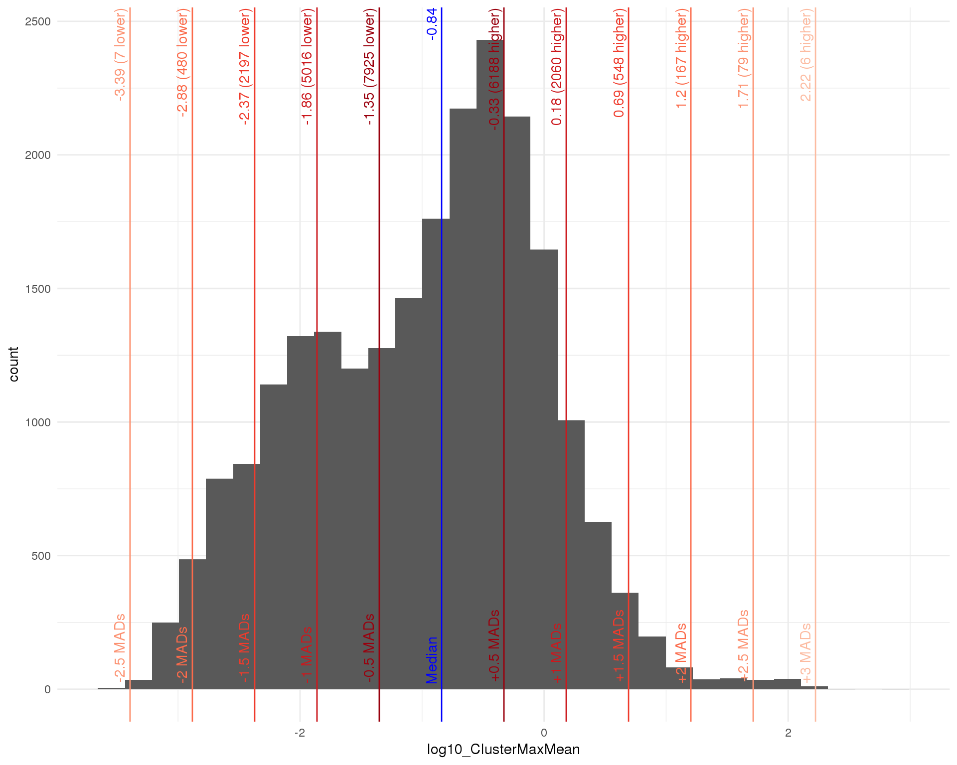
Expand here to see past versions of filter-1.png:
| Version | Author | Date |
|---|---|---|
| b610506 | Luke Zappia | 2019-02-27 |
maxmean_mads  <- 0.5
maxmean_out   <- isOutlier(rowData(sce)$log10_ClusterMaxMean,
                           nmads = maxmean_mads, type = "lower")
maxmean_thresh <- attr(maxmean_out, "thresholds")["lower"]

sce_filt <- sce[rowData(sce)$log10_ClusterMaxMean > maxmean_thresh, ]
Selecting a threshold of -1.3505126 removes 7925 genes.
Fitting
We will use edgeR for differential expression testing to identify marker genes for our clusters. Although originally designed for bulk RNA-seq comparisons have shown that edgeR also has good performance for scRNA-seq. We will test each cluster against all the other cells in the dataset. This may miss subtler differences between similar cell types but should identify key markers for each cluster and is computationally easier than completing every pairwise comparison.
First we construct a design matrix and DGEList object then we calculate normalisation factors, estimate dispersions and fit the model.
# Cell detection rate
det_rate <- scale(Matrix::colMeans(counts(sce_filt) > 0))

# Create design matrix
design <- model.matrix(~ 0 + det_rate + colData(sce_filt)$Cluster)
colnames(design) <- c("DetRate", paste0("C", seq_len(n_clusts) - 1))

# Create DGEList
dge <- DGEList(counts(sce_filt))
# Add gene annotation
dge$genes <- rowData(sce_filt)[, c("Name", "ID", "entrezgene", "description")]
# Calculate norm factors
dge <- calcNormFactors(dge)
# Estimate dispersions
dge <- estimateDisp(dge, design)
# Fit model
de_fit <- glmQLFit(dge, design = design)
Before we perform the tests let’s check how good the fit is.
Mean
plot_data <- tibble(Observed = log1p(Matrix::rowMeans(counts(sce_filt))),
                    Expected = log1p(rowMeans(de_fit$fitted.values))) %>%
    mutate(Mean = 0.5 * (Observed + Expected),
           Difference = Observed - Expected)

ggplot(plot_data, aes(x = Mean, y = Difference)) +
    geom_point() +
    geom_smooth(method = "loess") +
    geom_hline(yintercept = 0, colour = "red") +
    xlab("0.5 * (Observed + Expected)") +
    ylab("Observed - Expected") +
    ggtitle("Fit of gene means") +
    theme_minimal()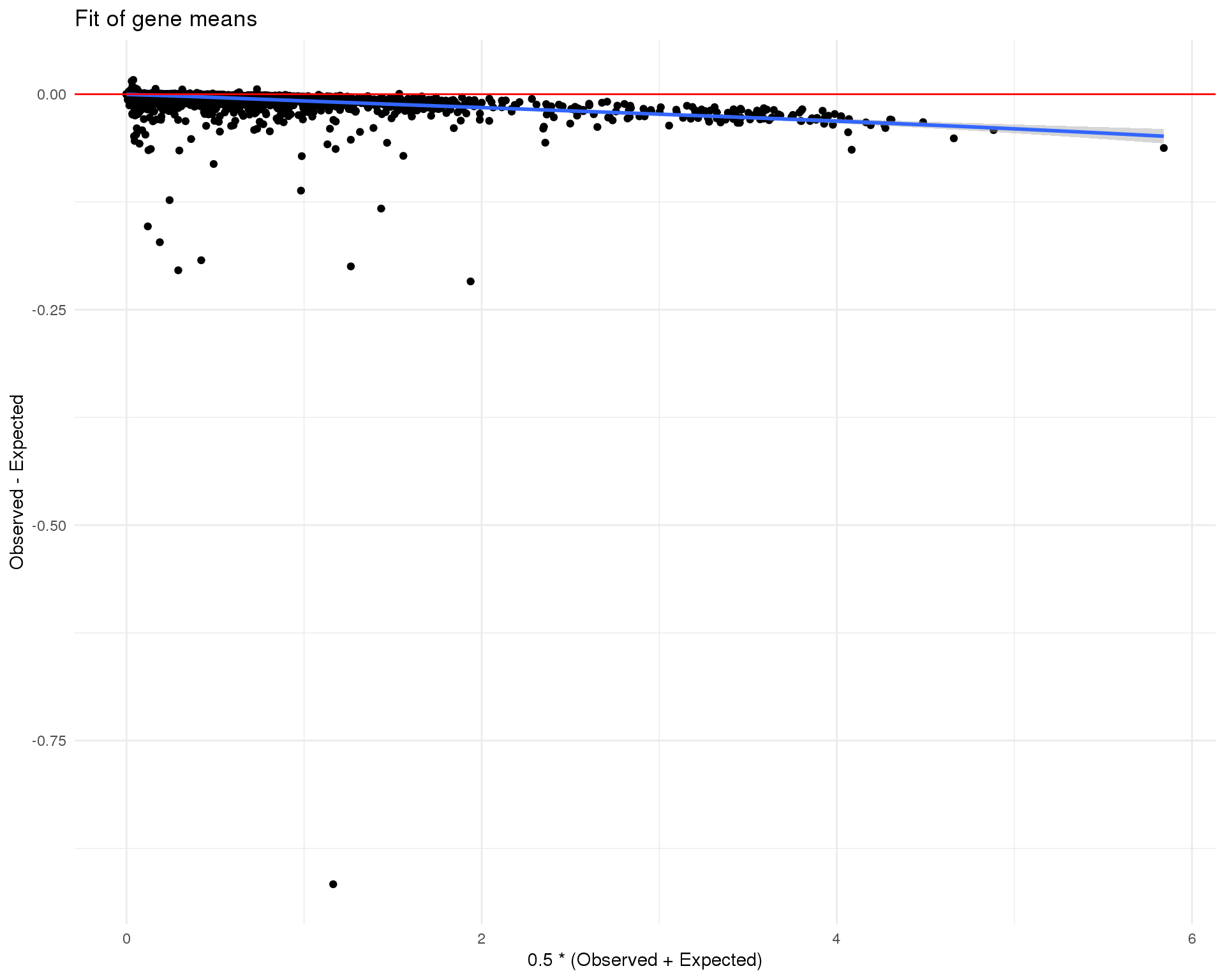
Zeros
plot_data <- tibble(Observed = Matrix::rowMeans(counts(sce_filt) == 0),
                    Expected = rowMeans(
                        (1 + de_fit$fitted.values * dge$tagwise.dispersion) ^
                            (-1 / dge$tagwise.dispersion)
                    )) %>%
    mutate(Mean = 0.5 * (Observed + Expected),
           Difference = Observed - Expected)

ggplot(plot_data, aes(x = Mean, y = Difference)) +
    geom_point() +
    geom_smooth(method = "loess") +
    geom_hline(yintercept = 0, colour = "red") +
    xlab("0.5 * (Observed + Expected)") +
    ylab("Observed - Expected") +
    ggtitle("Fit of gene proportion of zeros") +
    theme_minimal()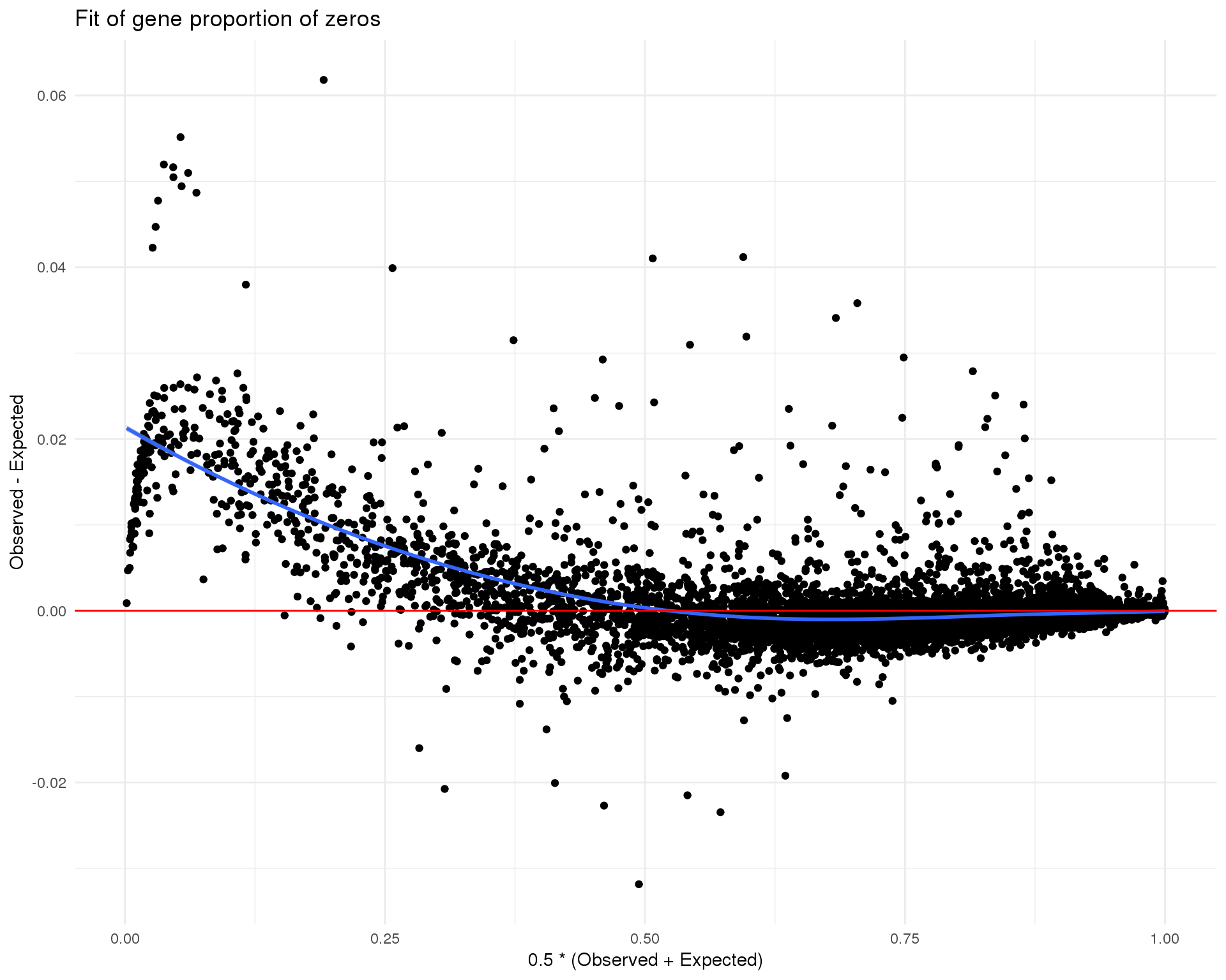
BCV
plotBCV(dge)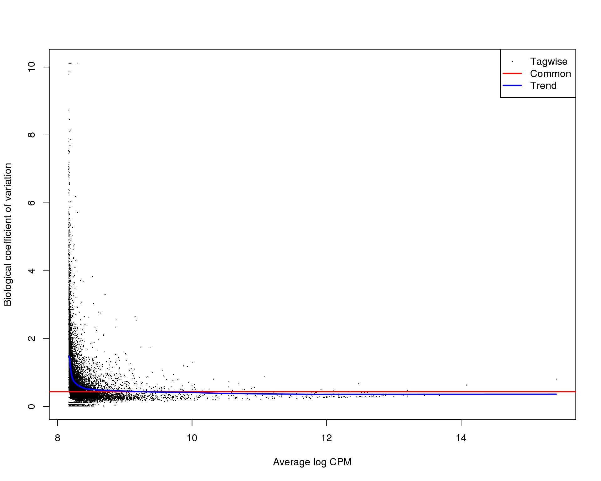
QL Dispersions
plotQLDisp(de_fit)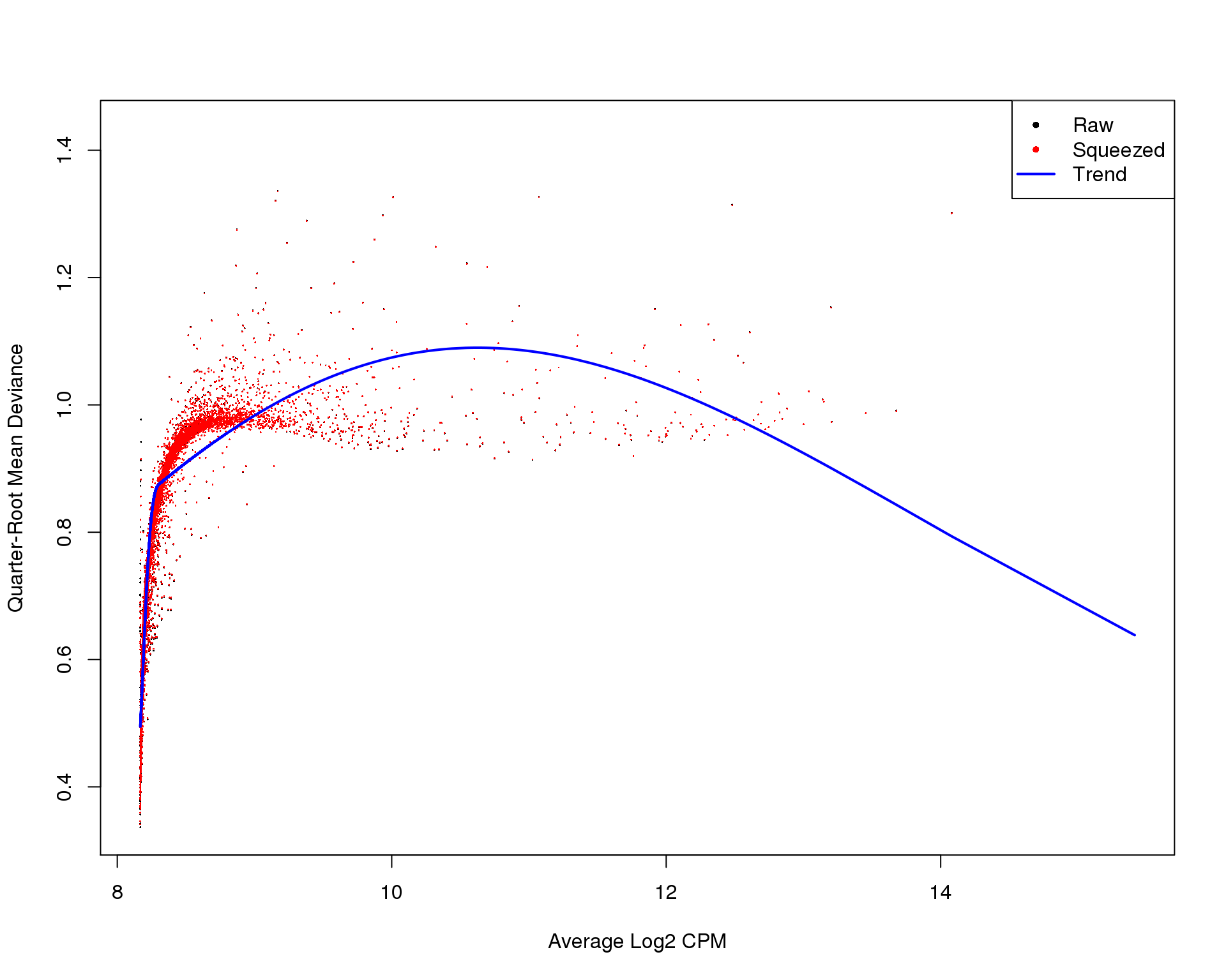
Expand here to see past versions of qldisp-1.png:
| Version | Author | Date |
|---|---|---|
| b610506 | Luke Zappia | 2019-02-27 |
| 8f826ef | Luke Zappia | 2019-02-08 |
These plots suggest that the fit is fairly good and there isn’t an excessive amount of zero inflation we would need to account for using other methods.
Testing
Once we have a fitted model we can test each of our contrasts.
de_tests <- bplapply(seq_len(n_clusts), function(idx) {
    contrast <- rep(-1 / (n_clusts - 1), n_clusts)
    contrast[idx] <- 1
    contrast <- c(0, contrast)
    glmQLFTest(de_fit, contrast = contrast)
}, BPPARAM = bpparam5)
de_list <- lapply(seq_len(n_clusts), function(idx) {
topTags(de_tests[[idx]], n = Inf, sort.by = "logFC")$table %>%
as.data.frame() %>%
mutate(Cluster = idx - 1) %>%
select(Cluster, everything())
})
names(de_list) <- paste("Cluster", 0:(n_clusts - 1))
fdr_thresh <- 0.05
logFC_thresh <- 1
markers_list <- lapply(de_list, function(de) {
de %>%
filter(FDR < fdr_thresh, logFC > logFC_thresh) %>%
select(Name, logFC, PValue, FDR)
})Before we look at the gene lists let’s check some diagnostic plots.
P-values
Distribution of p-values for each cluster should be uniform with a peak near zero.
src_list <- lapply(seq_len(n_clusts) - 1, function(clust) {
    src <- c(
        "### Cluster {{clust}} {.unnumbered}",
        "```{r pvals-{{clust}}}",
        "ggplot(de_list[[{{clust}} + 1]], aes(x = PValue)) +",
        "geom_histogram() +",
        "theme_minimal()",
        "```",
        ""
    )
    knit_expand(text = src)
})

out <- knit_child(text = unlist(src_list), options = list(cache = FALSE))
Cluster 0
ggplot(de_list[[0 + 1]], aes(x = PValue)) +
geom_histogram() +
theme_minimal()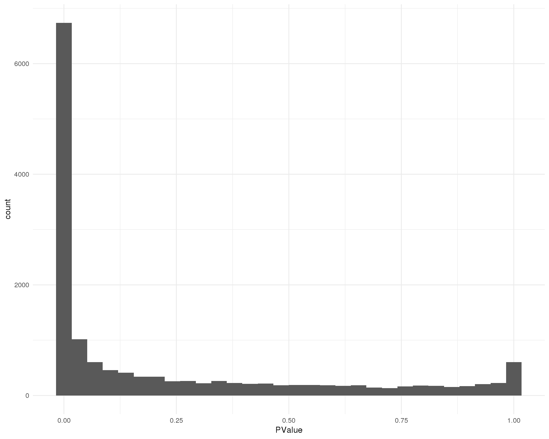
Cluster 1
ggplot(de_list[[1 + 1]], aes(x = PValue)) +
geom_histogram() +
theme_minimal()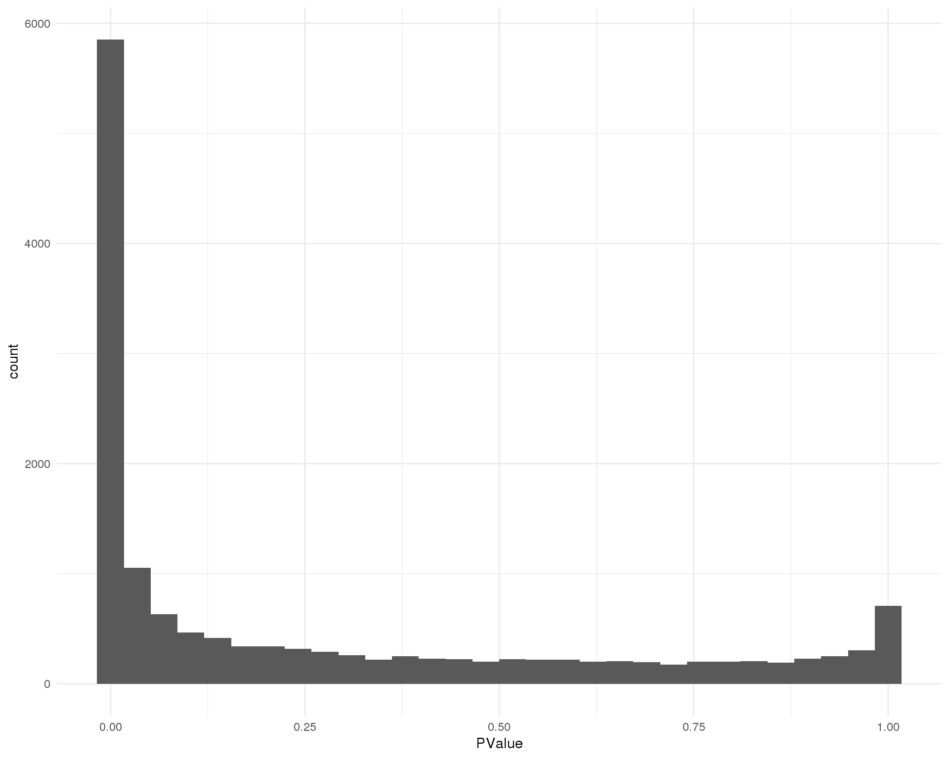
Cluster 2
ggplot(de_list[[2 + 1]], aes(x = PValue)) +
geom_histogram() +
theme_minimal()
Cluster 3
ggplot(de_list[[3 + 1]], aes(x = PValue)) +
geom_histogram() +
theme_minimal()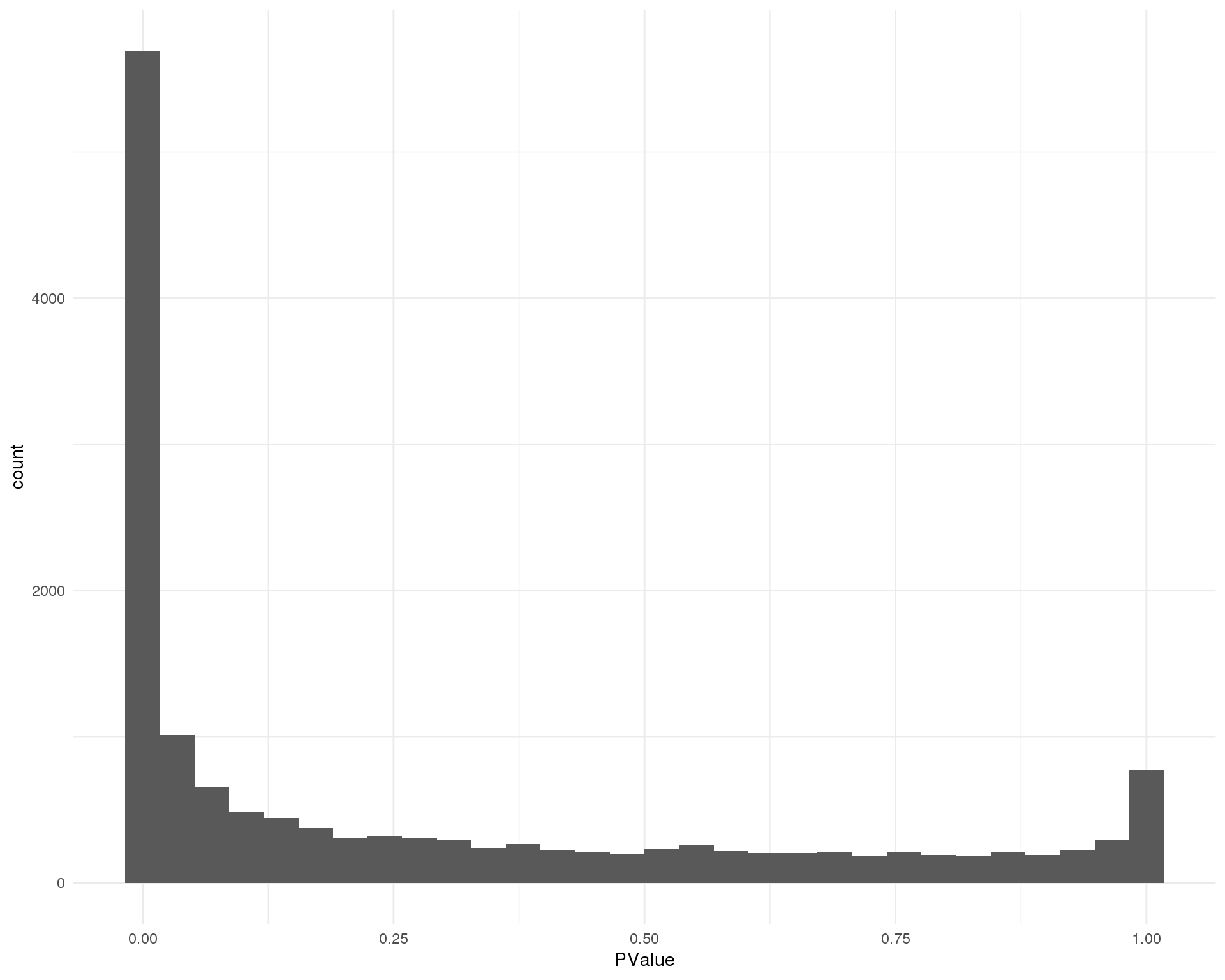
Cluster 4
ggplot(de_list[[4 + 1]], aes(x = PValue)) +
geom_histogram() +
theme_minimal()
Cluster 5
ggplot(de_list[[5 + 1]], aes(x = PValue)) +
geom_histogram() +
theme_minimal()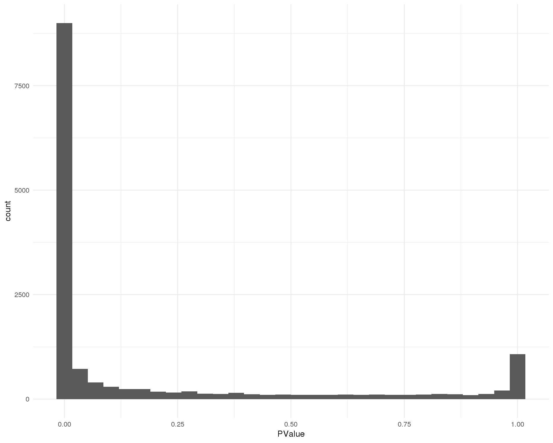
Cluster 6
ggplot(de_list[[6 + 1]], aes(x = PValue)) +
geom_histogram() +
theme_minimal()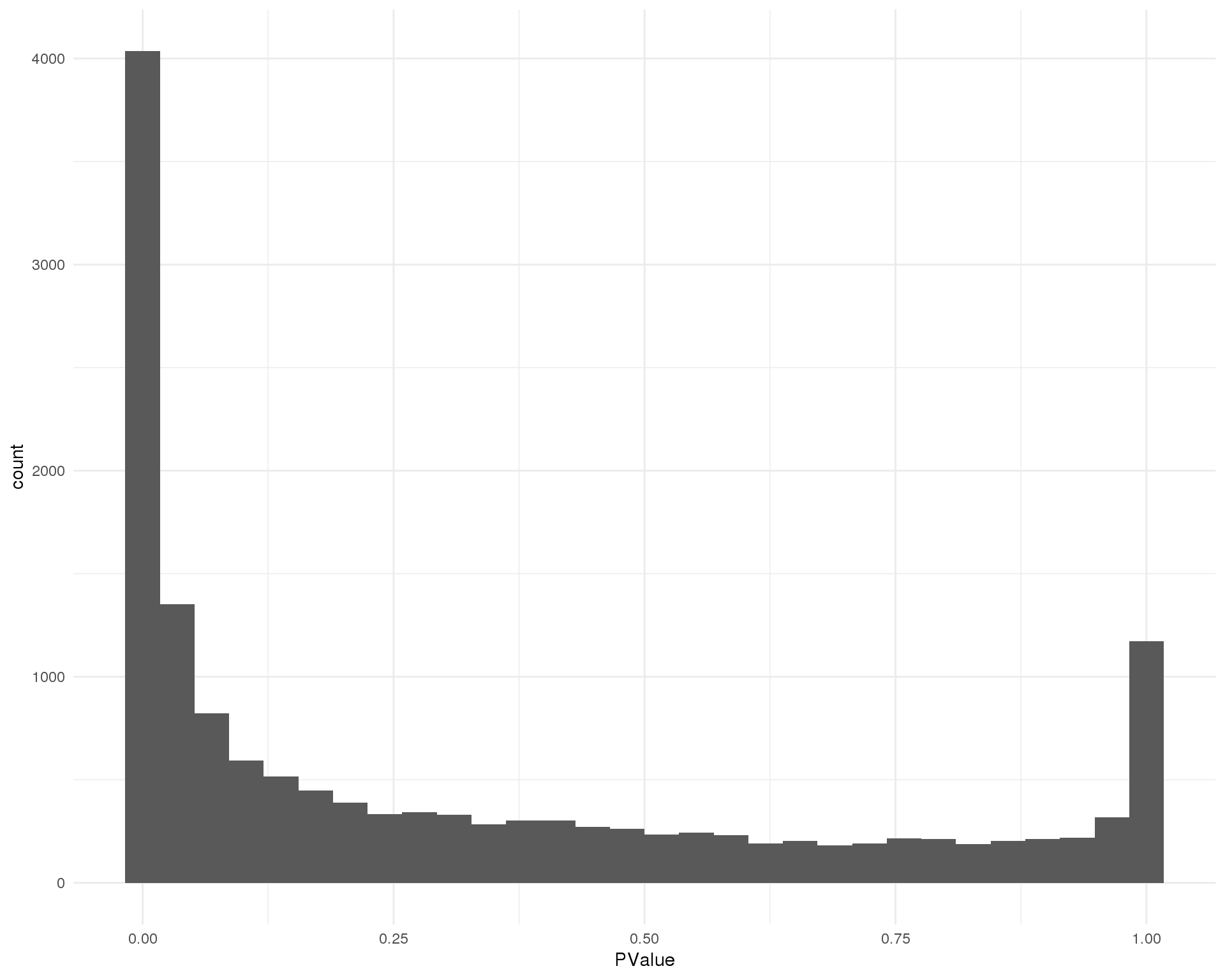
Cluster 7
ggplot(de_list[[7 + 1]], aes(x = PValue)) +
geom_histogram() +
theme_minimal()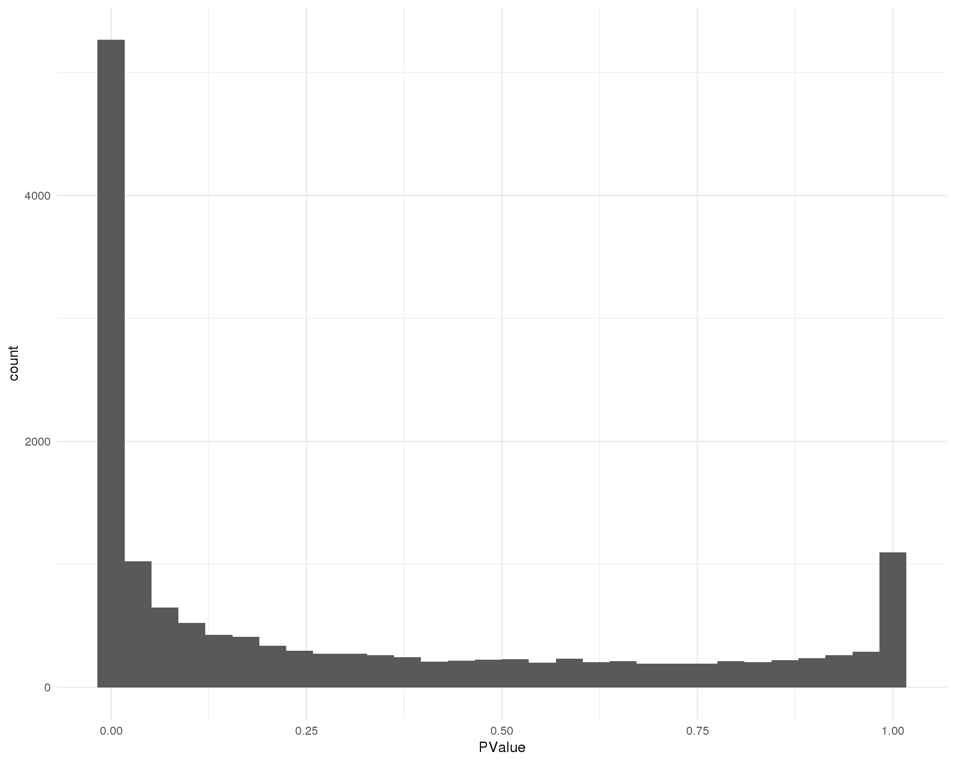
Cluster 8
ggplot(de_list[[8 + 1]], aes(x = PValue)) +
geom_histogram() +
theme_minimal()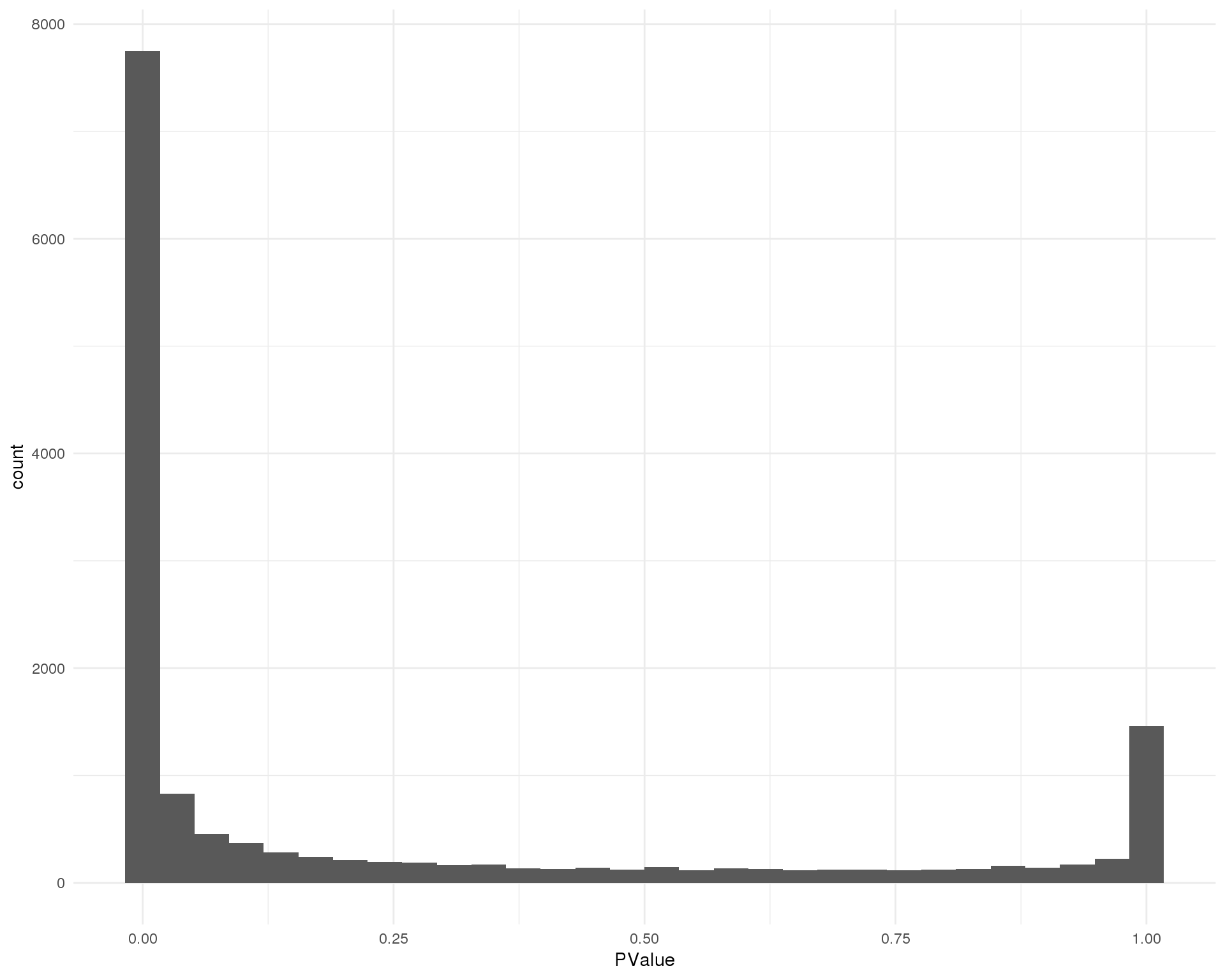
Cluster 9
ggplot(de_list[[9 + 1]], aes(x = PValue)) +
geom_histogram() +
theme_minimal()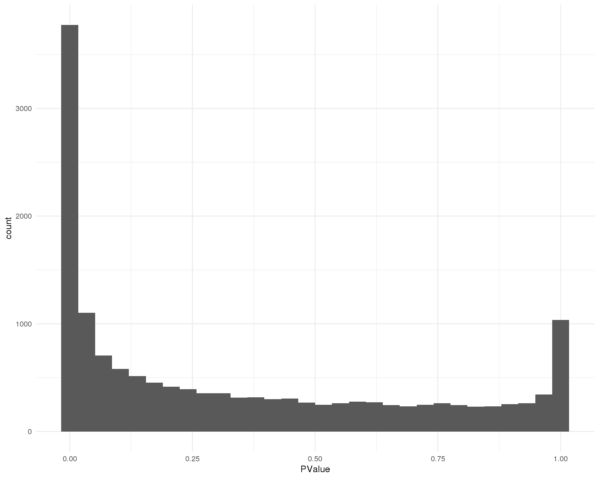
Cluster 10
ggplot(de_list[[10 + 1]], aes(x = PValue)) +
geom_histogram() +
theme_minimal()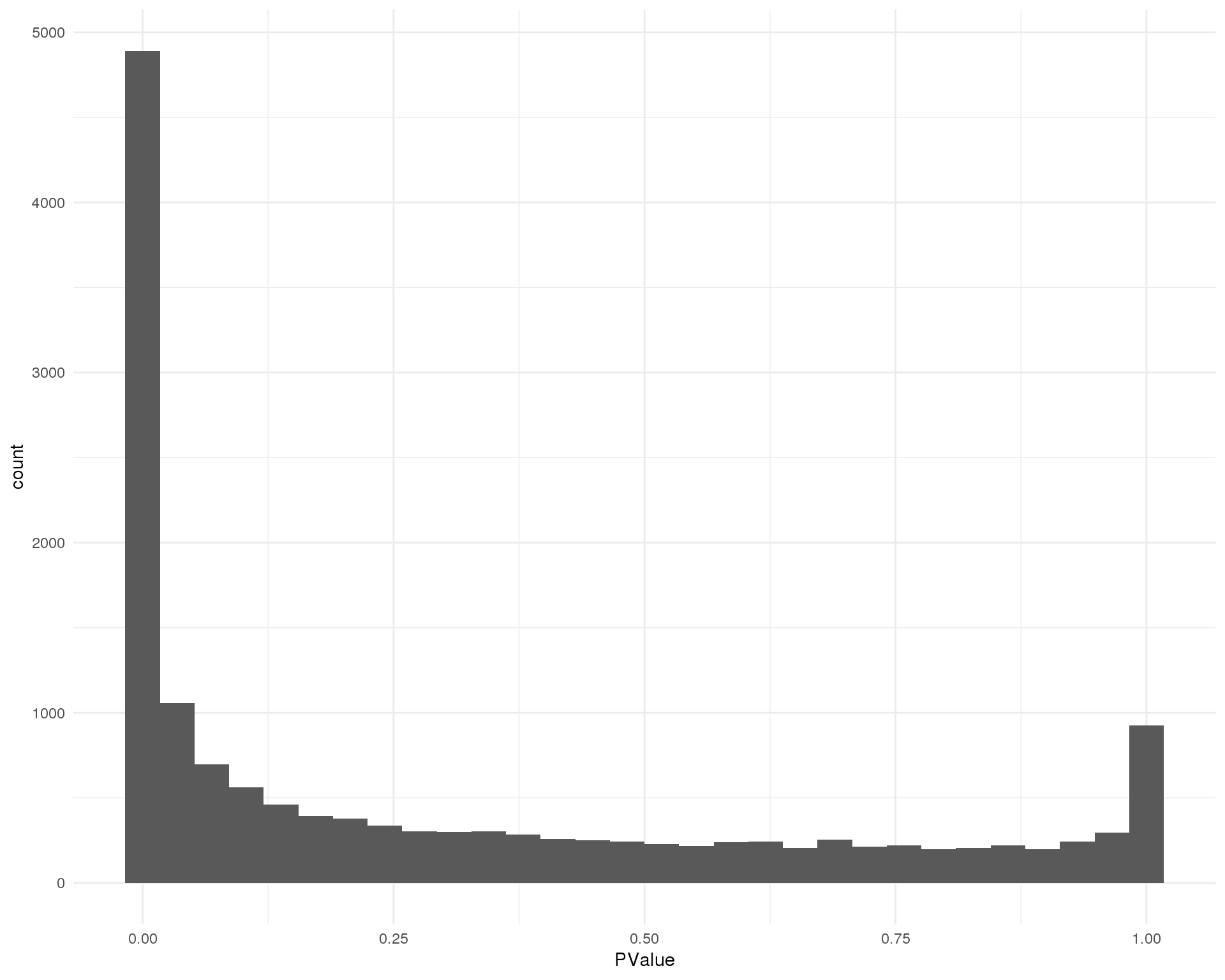
Cluster 11
ggplot(de_list[[11 + 1]], aes(x = PValue)) +
geom_histogram() +
theme_minimal()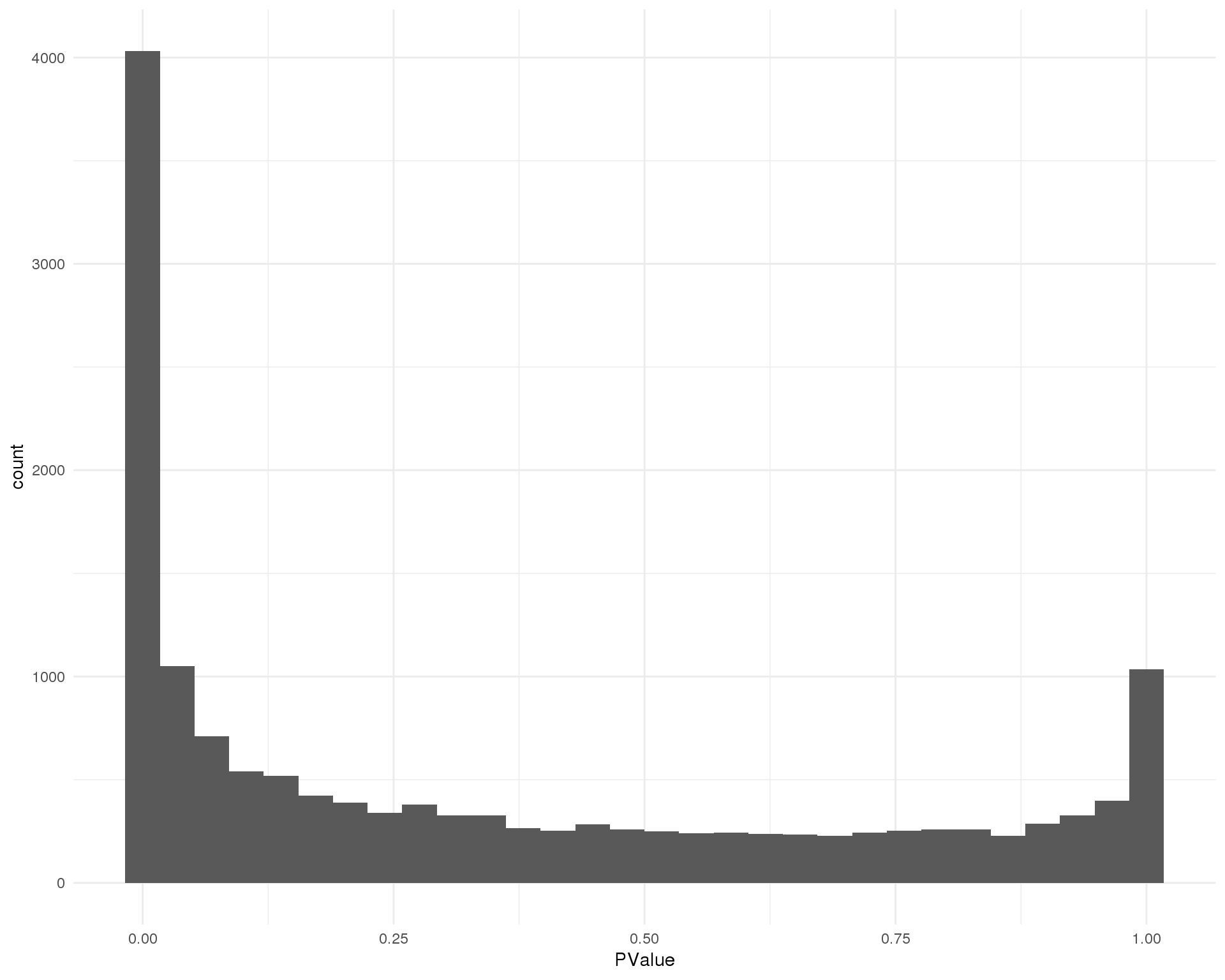
Cluster 12
ggplot(de_list[[12 + 1]], aes(x = PValue)) +
geom_histogram() +
theme_minimal()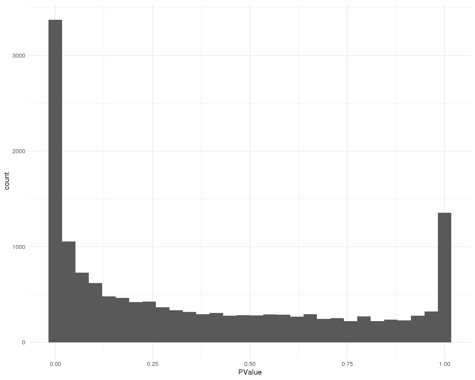
Expand here to see past versions of pvals-12-1.png:
| Version | Author | Date |
|---|---|---|
| b610506 | Luke Zappia | 2019-02-27 |
Mean-difference
Mean-difference plot highlighting significant genes.
src_list <- lapply(seq_len(n_clusts) - 1, function(clust) {
    src <- c(
        "### Cluster {{clust}} {.unnumbered}",
        "```{r md-{{clust}}}",
        "plotMD(de_tests[[{{clust}} + 1]])",
        "```",
        ""
    )
    knit_expand(text = src)
})

out <- knit_child(text = unlist(src_list), options = list(cache = FALSE))
Cluster 0
plotMD(de_tests[[0 + 1]])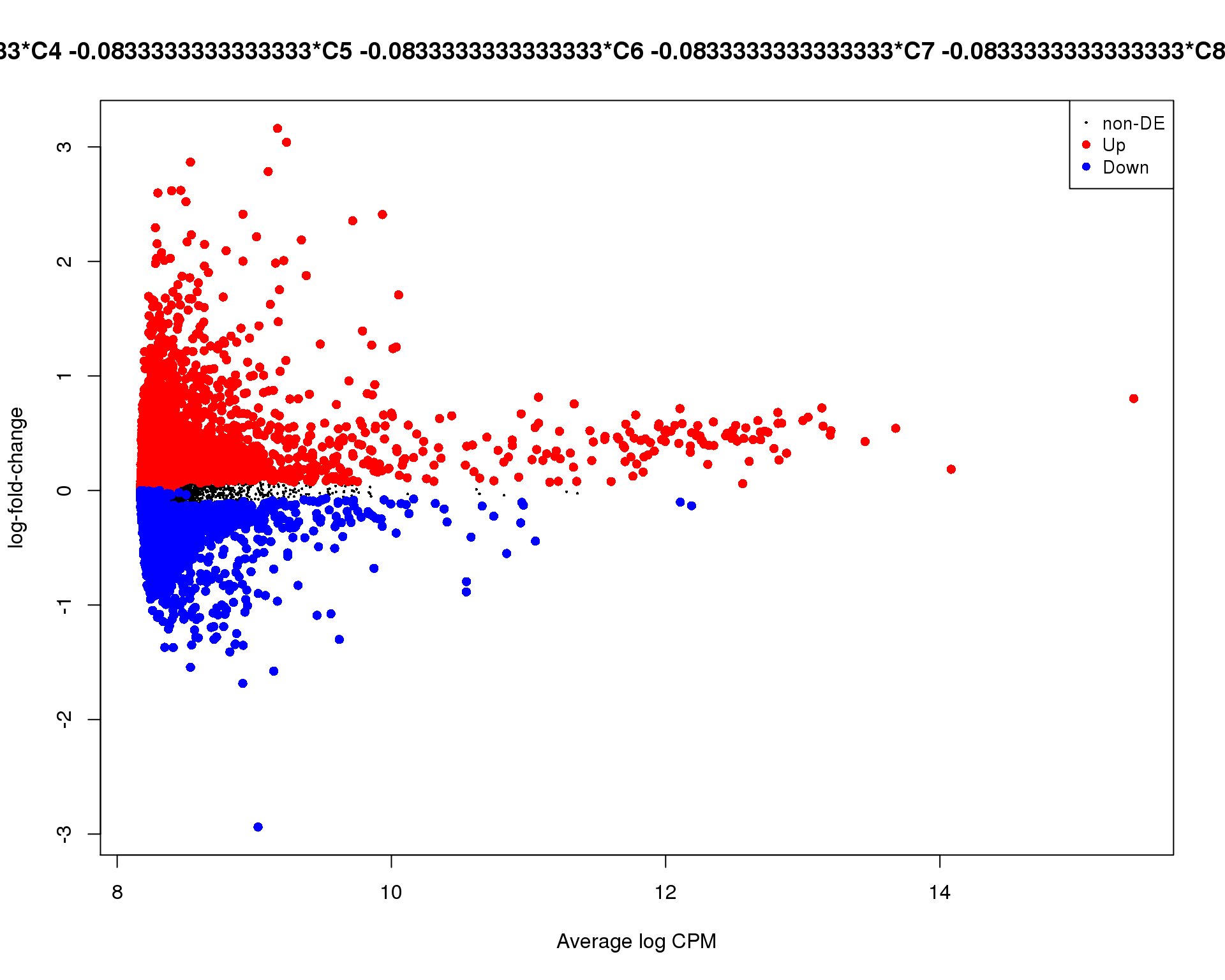
Cluster 1
plotMD(de_tests[[1 + 1]])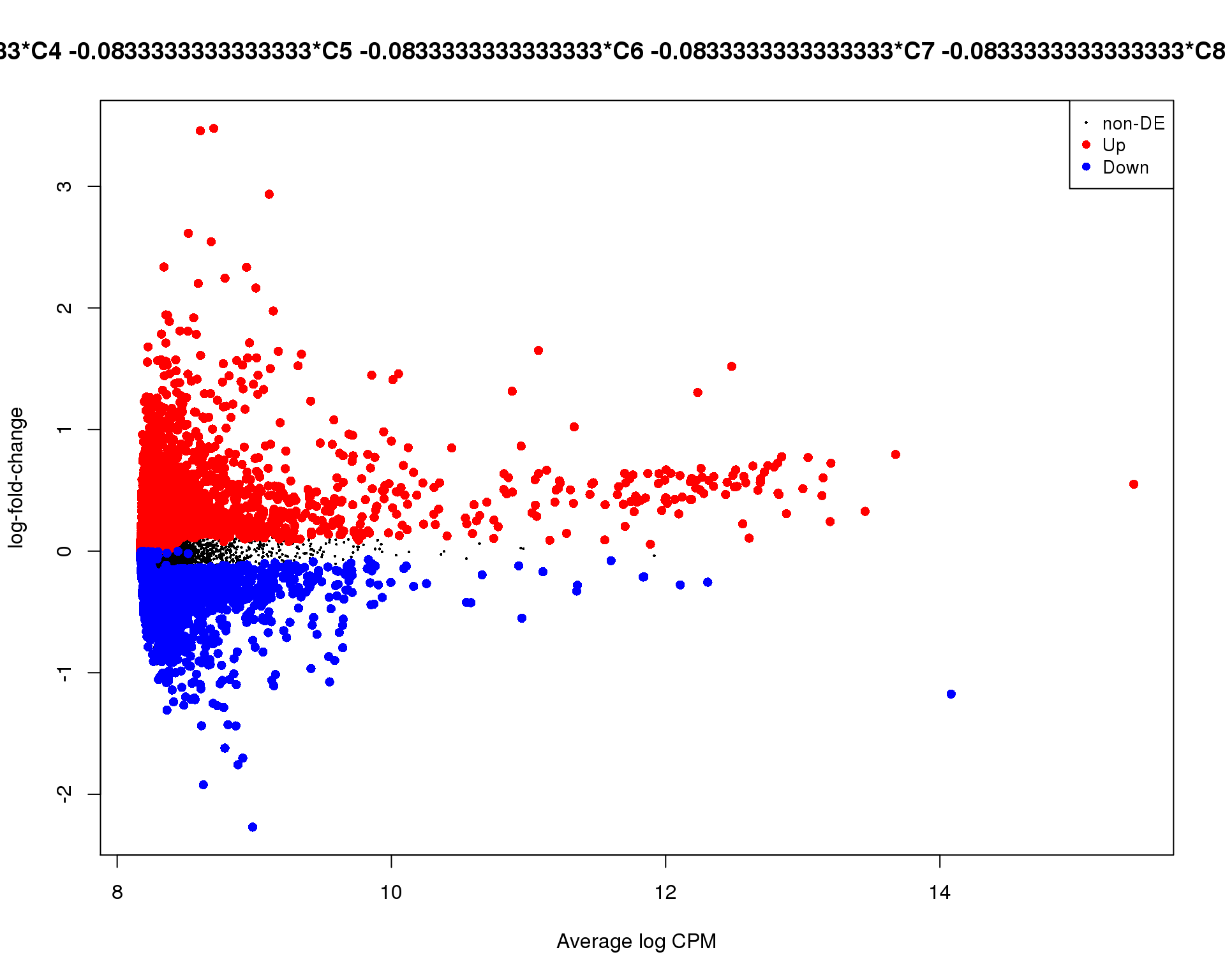
Cluster 2
plotMD(de_tests[[2 + 1]])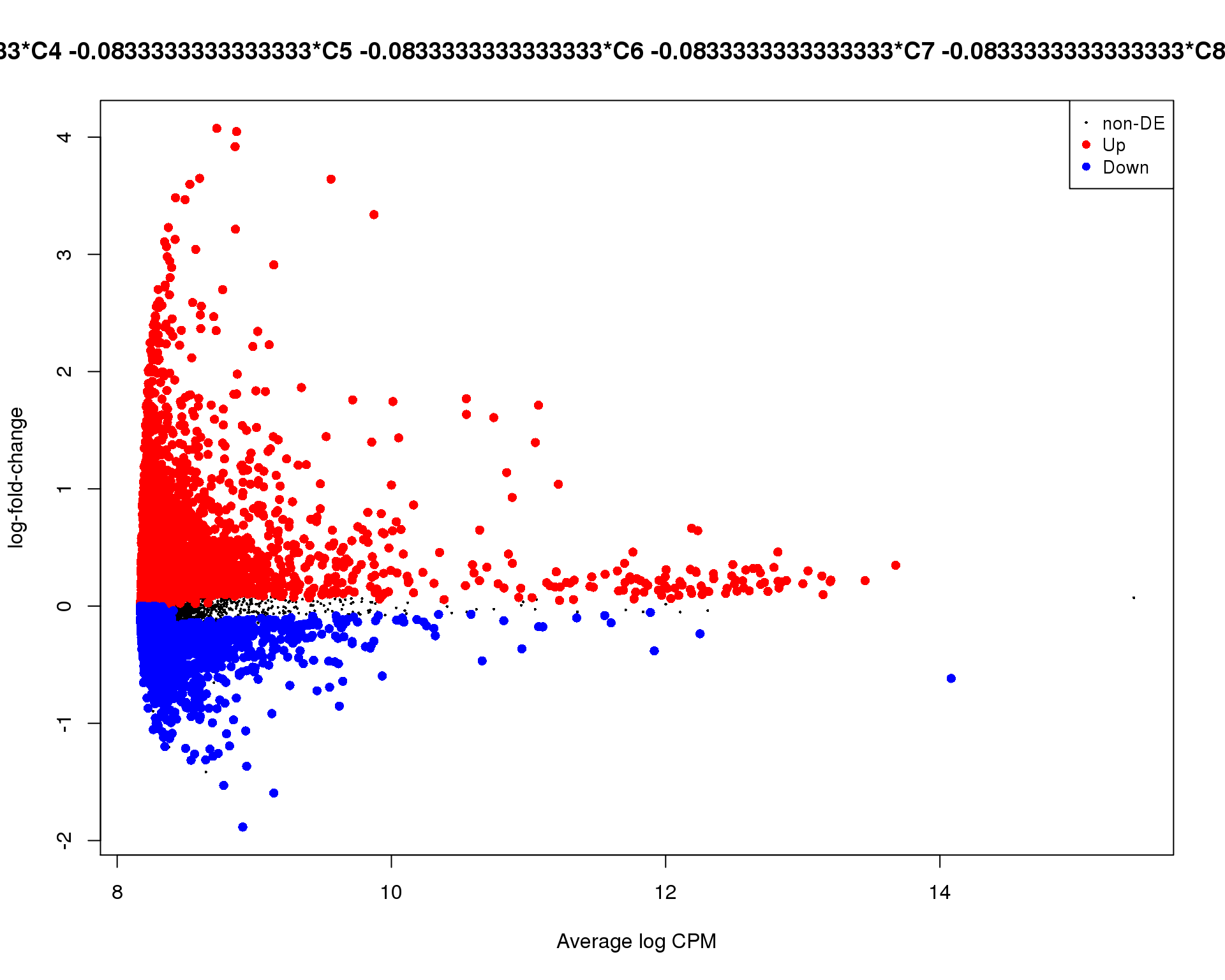
Cluster 3
plotMD(de_tests[[3 + 1]])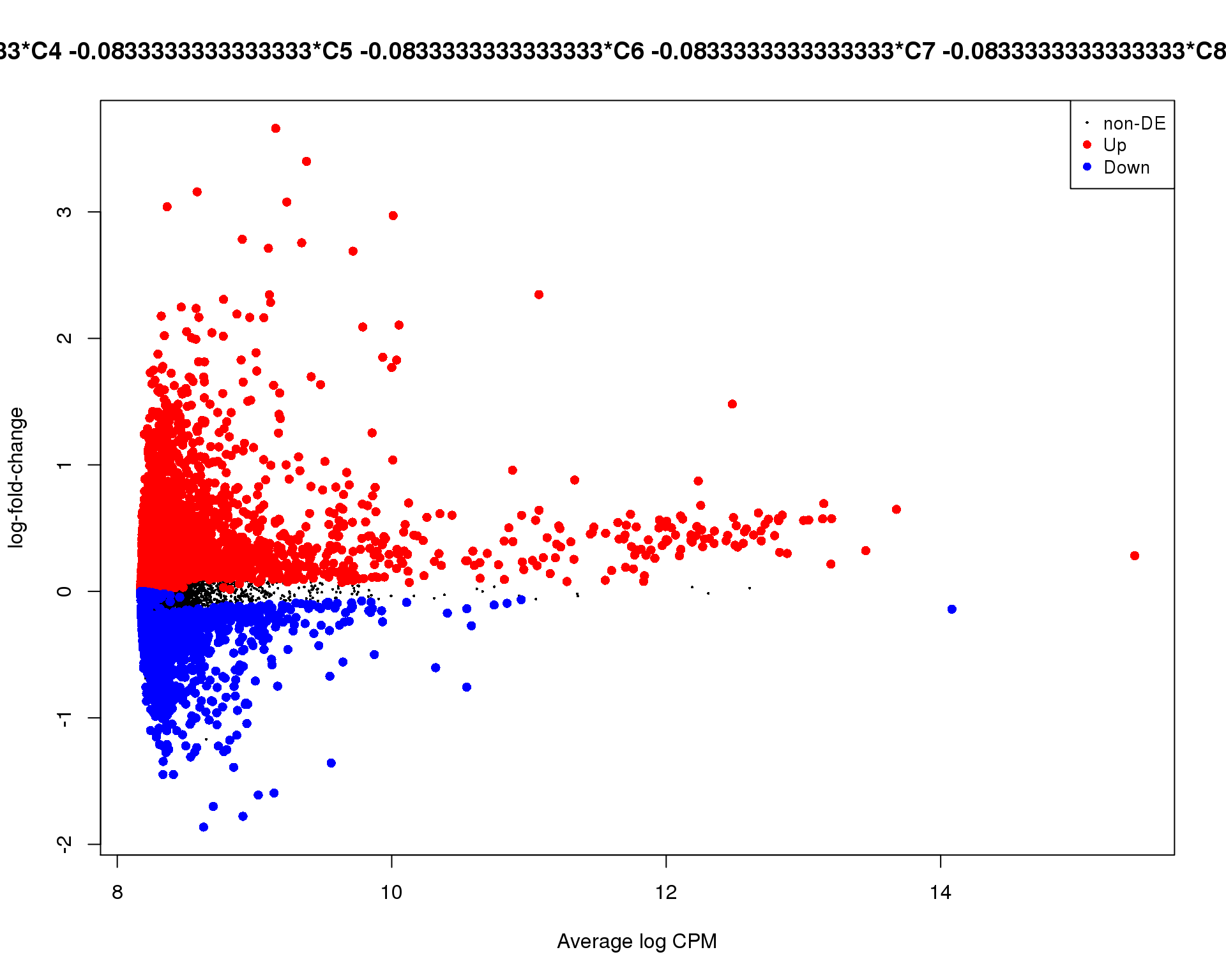
Cluster 4
plotMD(de_tests[[4 + 1]])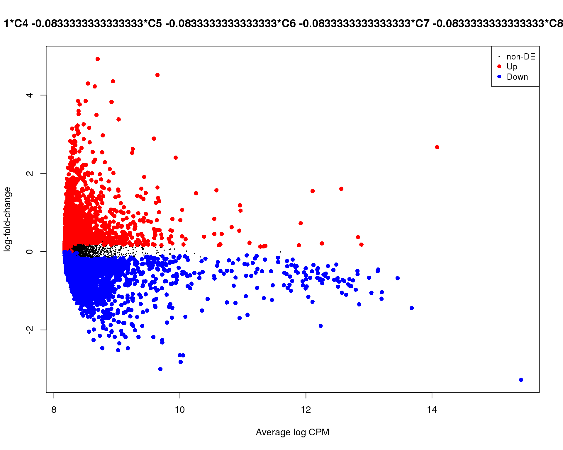
Cluster 5
plotMD(de_tests[[5 + 1]])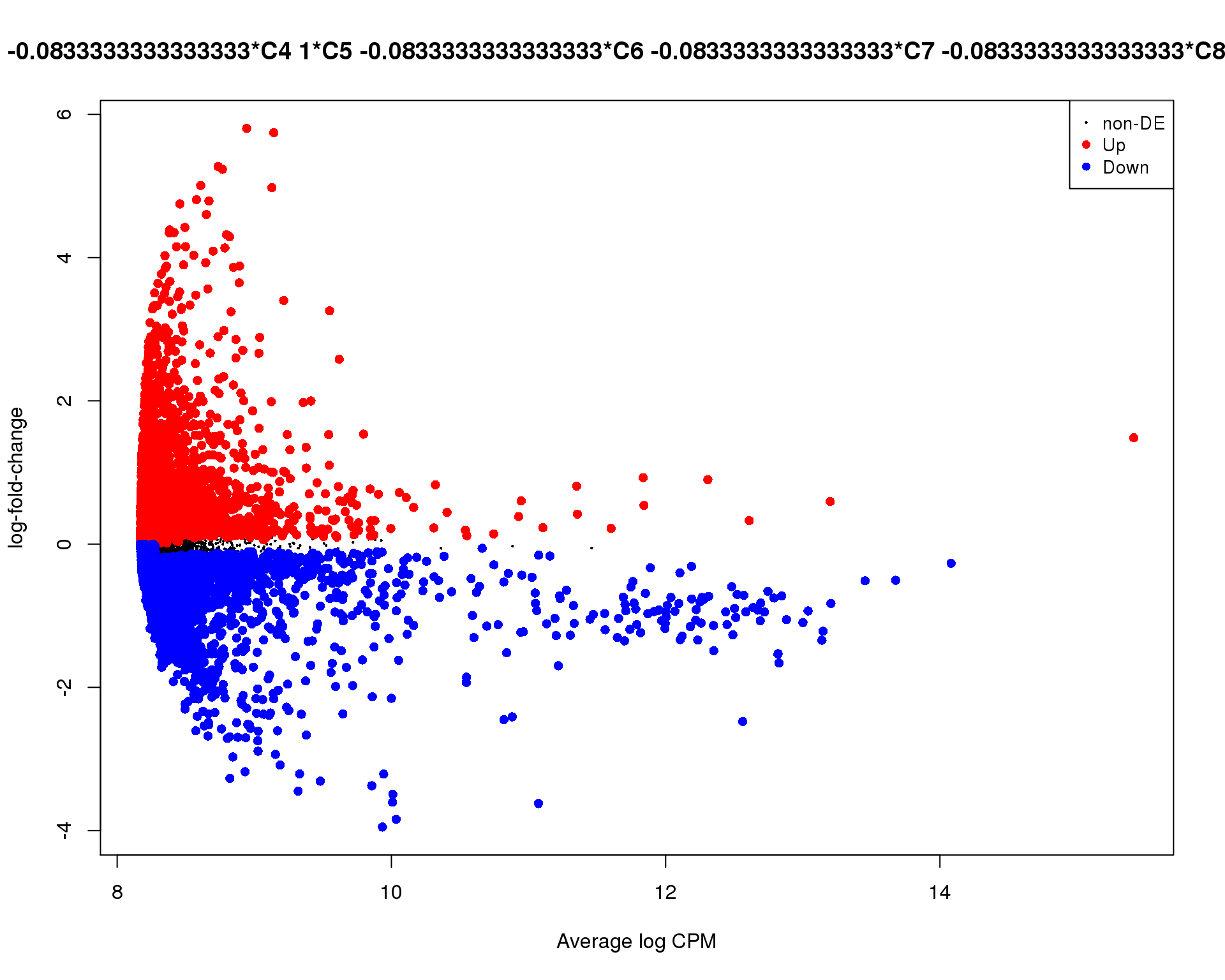
Cluster 6
plotMD(de_tests[[6 + 1]])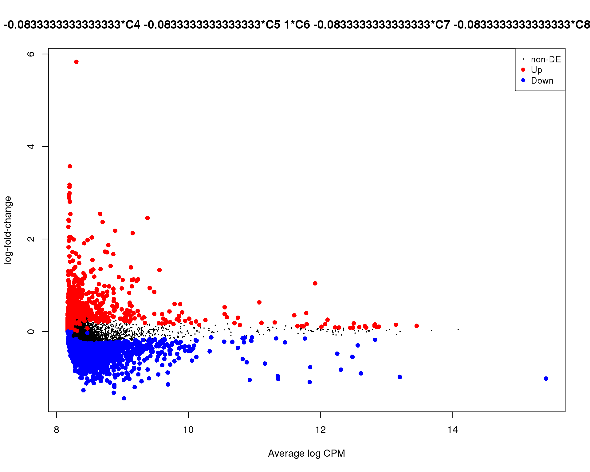
Cluster 7
plotMD(de_tests[[7 + 1]])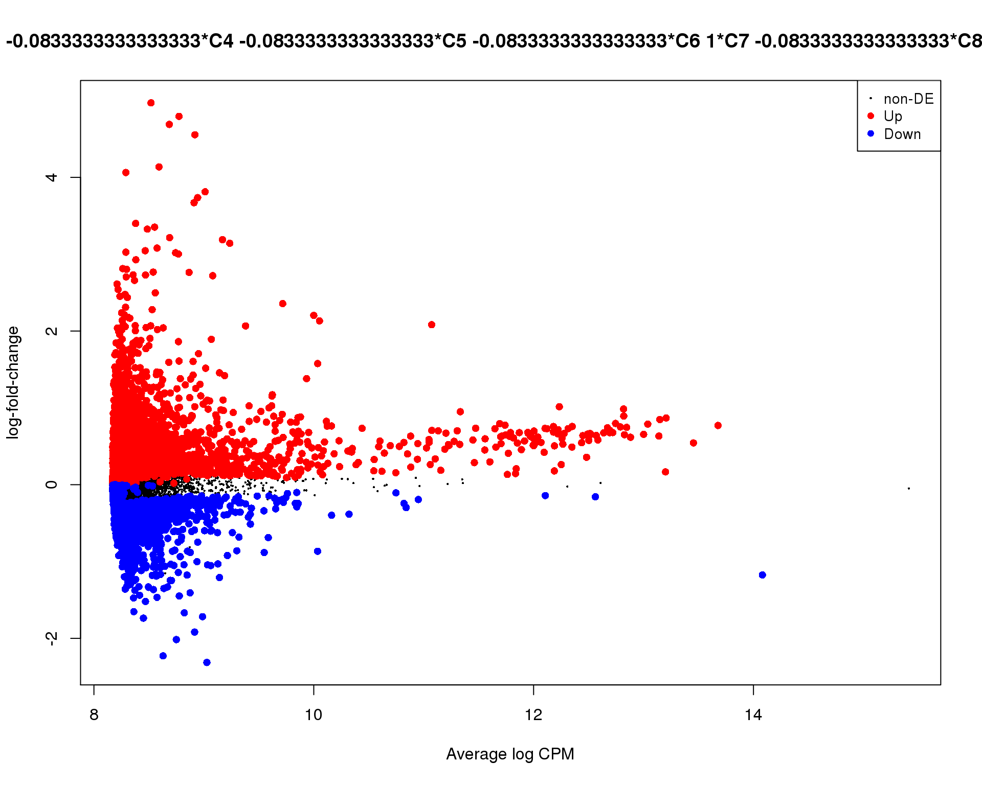
Cluster 8
plotMD(de_tests[[8 + 1]])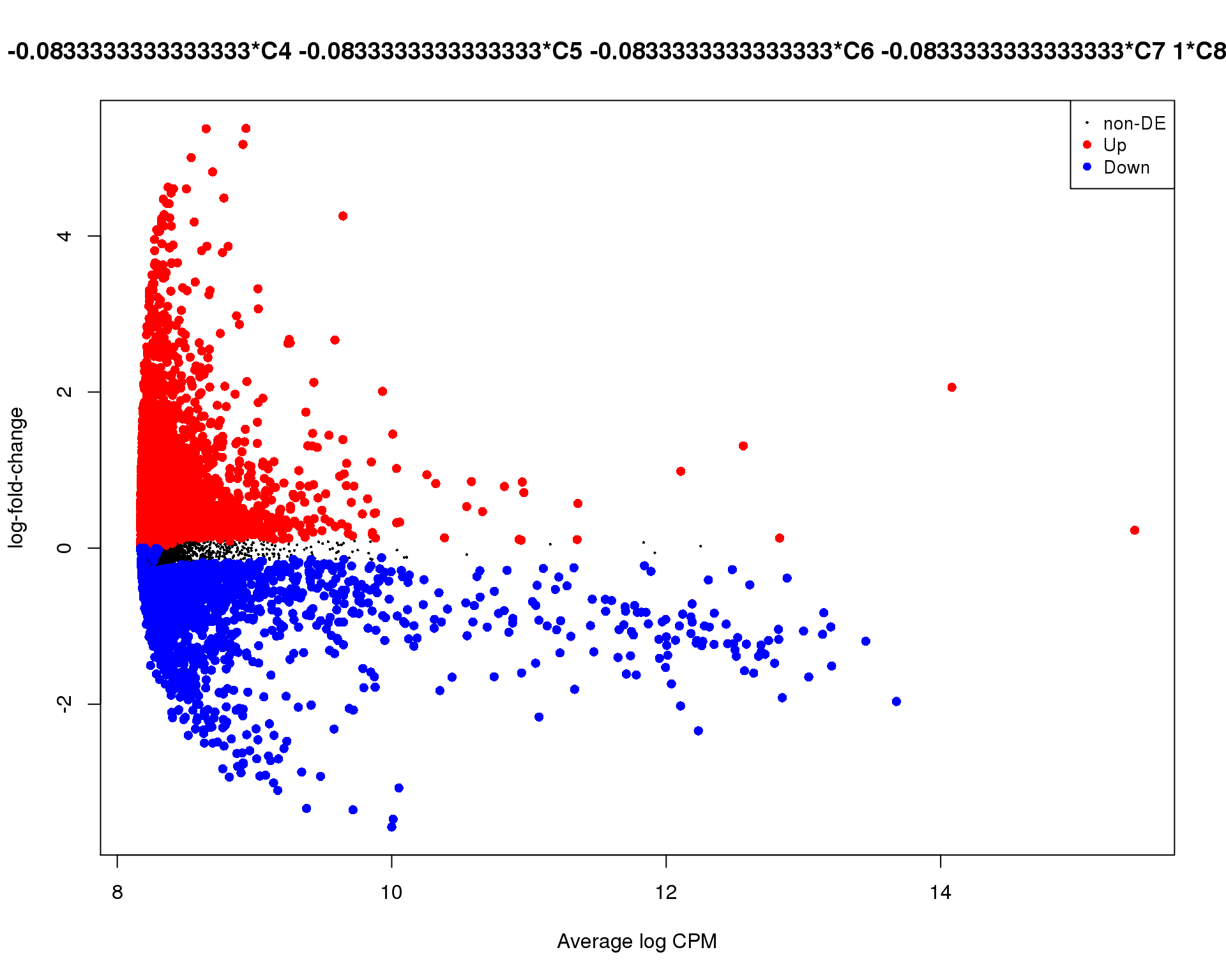
Cluster 9
plotMD(de_tests[[9 + 1]])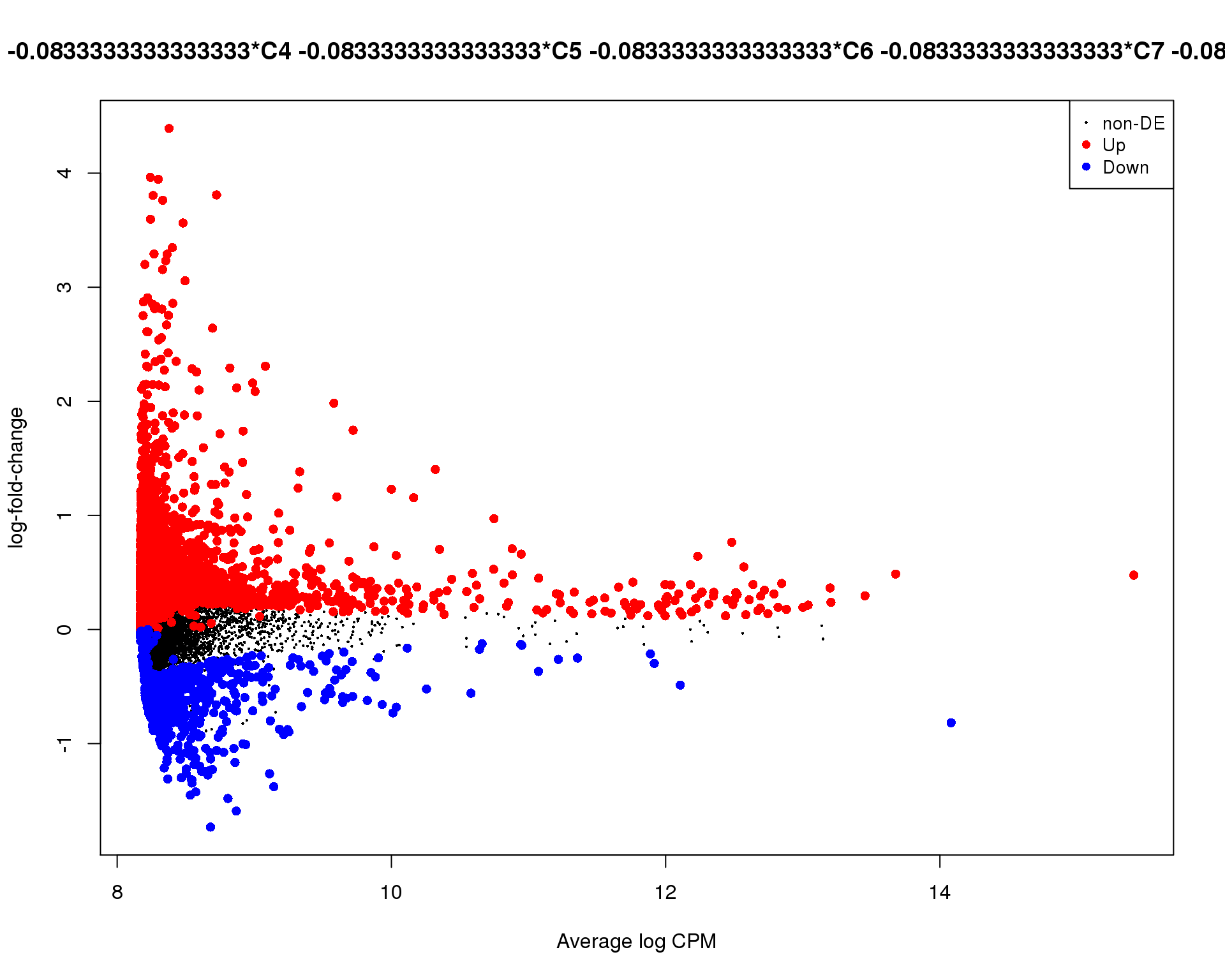
Cluster 10
plotMD(de_tests[[10 + 1]])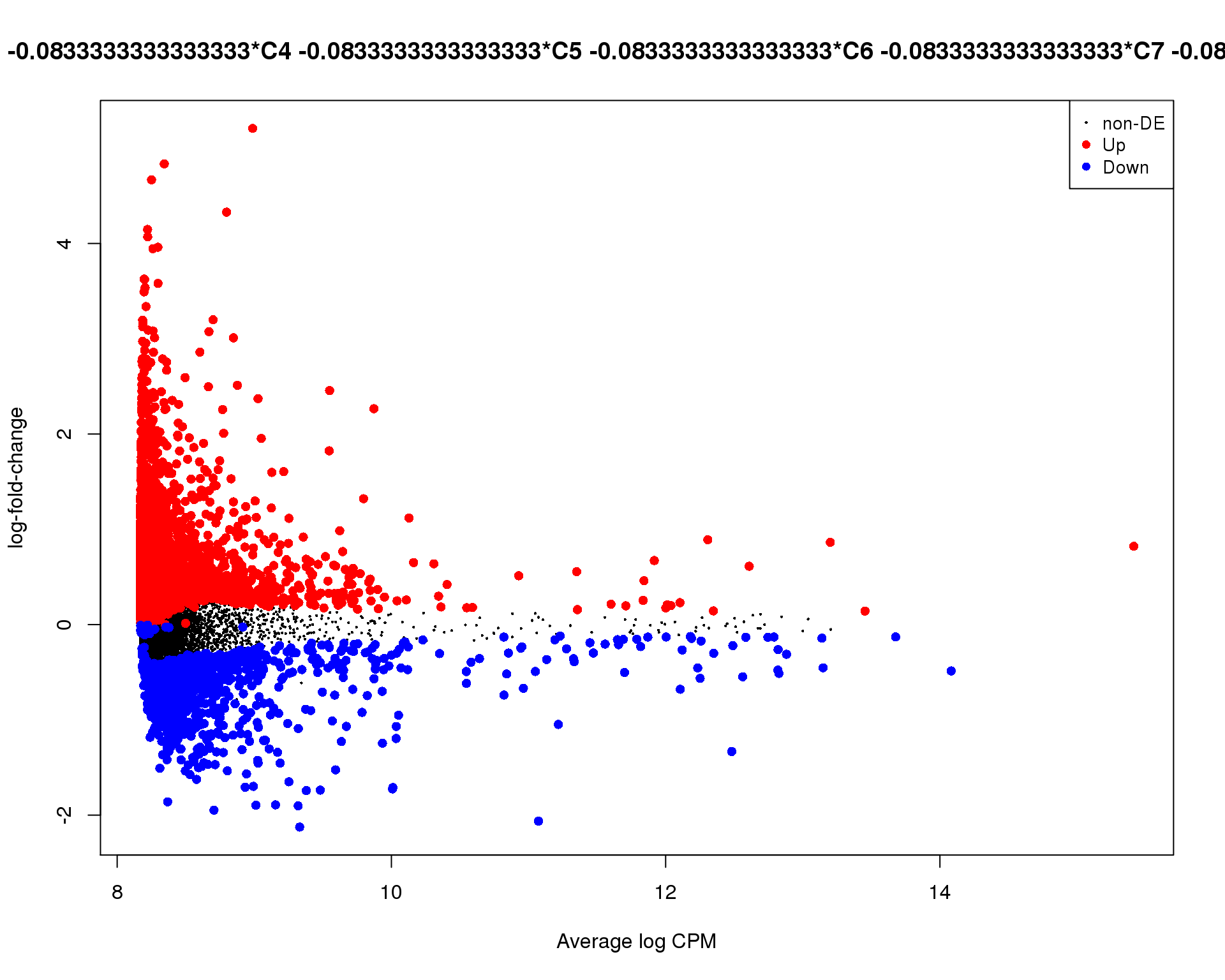
Cluster 11
plotMD(de_tests[[11 + 1]])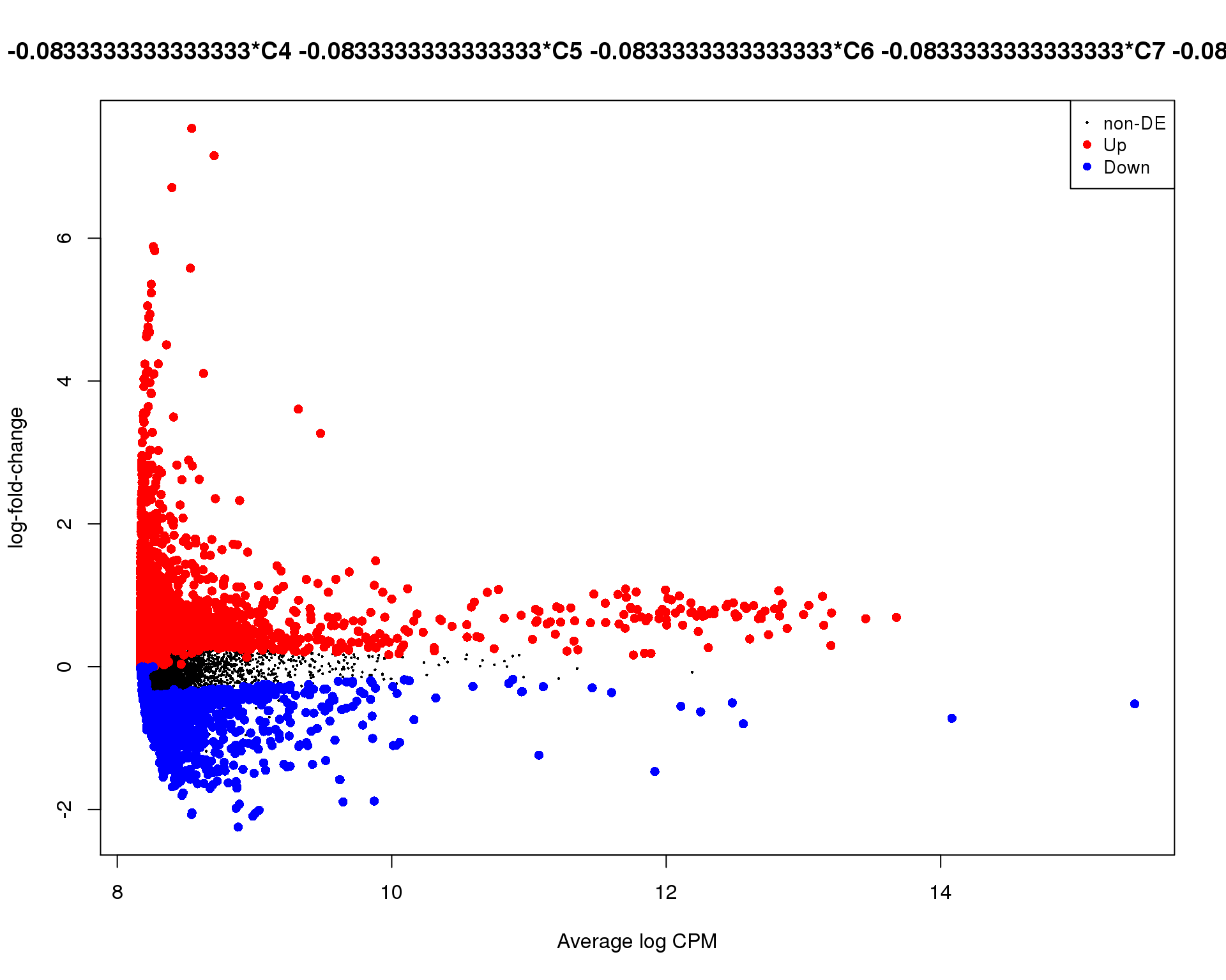
Cluster 12
plotMD(de_tests[[12 + 1]])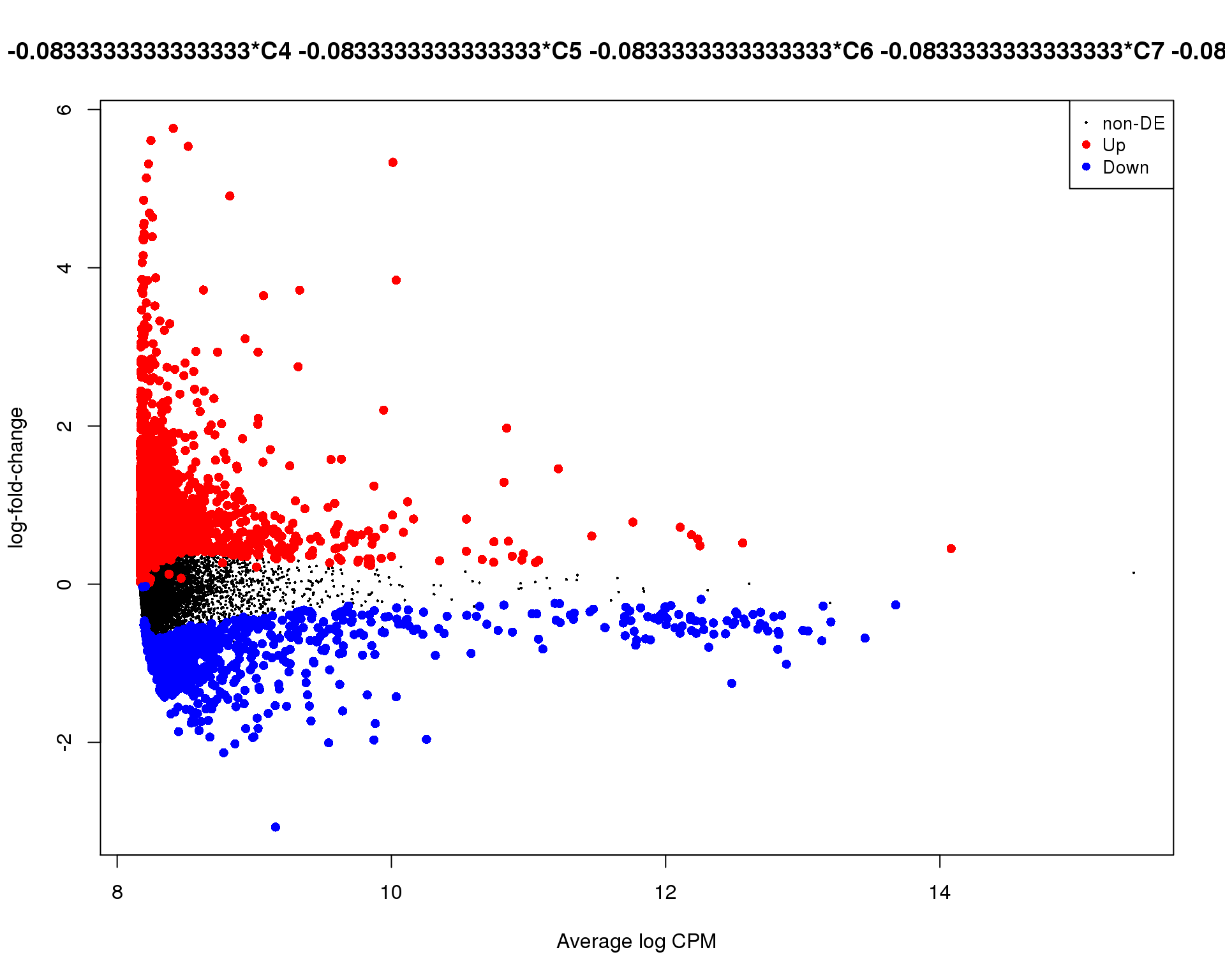
Expand here to see past versions of md-12-1.png:
| Version | Author | Date |
|---|---|---|
| b610506 | Luke Zappia | 2019-02-27 |
Summary
plot_data <- de_list %>%
    bind_rows() %>%
    filter(FDR < 0.05) %>%
    mutate(IsUp = logFC > 0) %>%
    group_by(Cluster) %>%
    summarise(Up = sum(IsUp), Down = sum(!IsUp)) %>%
    mutate(Down = -Down) %>%
    gather(key = "Direction", value = "Count", -Cluster) %>%
    mutate(Cluster = factor(Cluster, levels = 0:(n_clusts - 1)))

ggplot(plot_data,
       aes(x = fct_rev(Cluster), y = Count, fill = Direction)) +
    geom_col() +
    geom_text(aes(y = Count + sign(Count) * max(abs(Count)) * 0.07,
                  label = abs(Count)),
              size = 6, colour = "grey25") +
    coord_flip() +
    scale_fill_manual(values = c("#377eb8", "#e41a1c")) +
    ggtitle("Number of identified genes") +
    theme_minimal() +
    theme(axis.title = element_blank(),
          axis.line = element_blank(),
          axis.ticks = element_blank(),
          axis.text.x = element_blank(),
          legend.position = "bottom")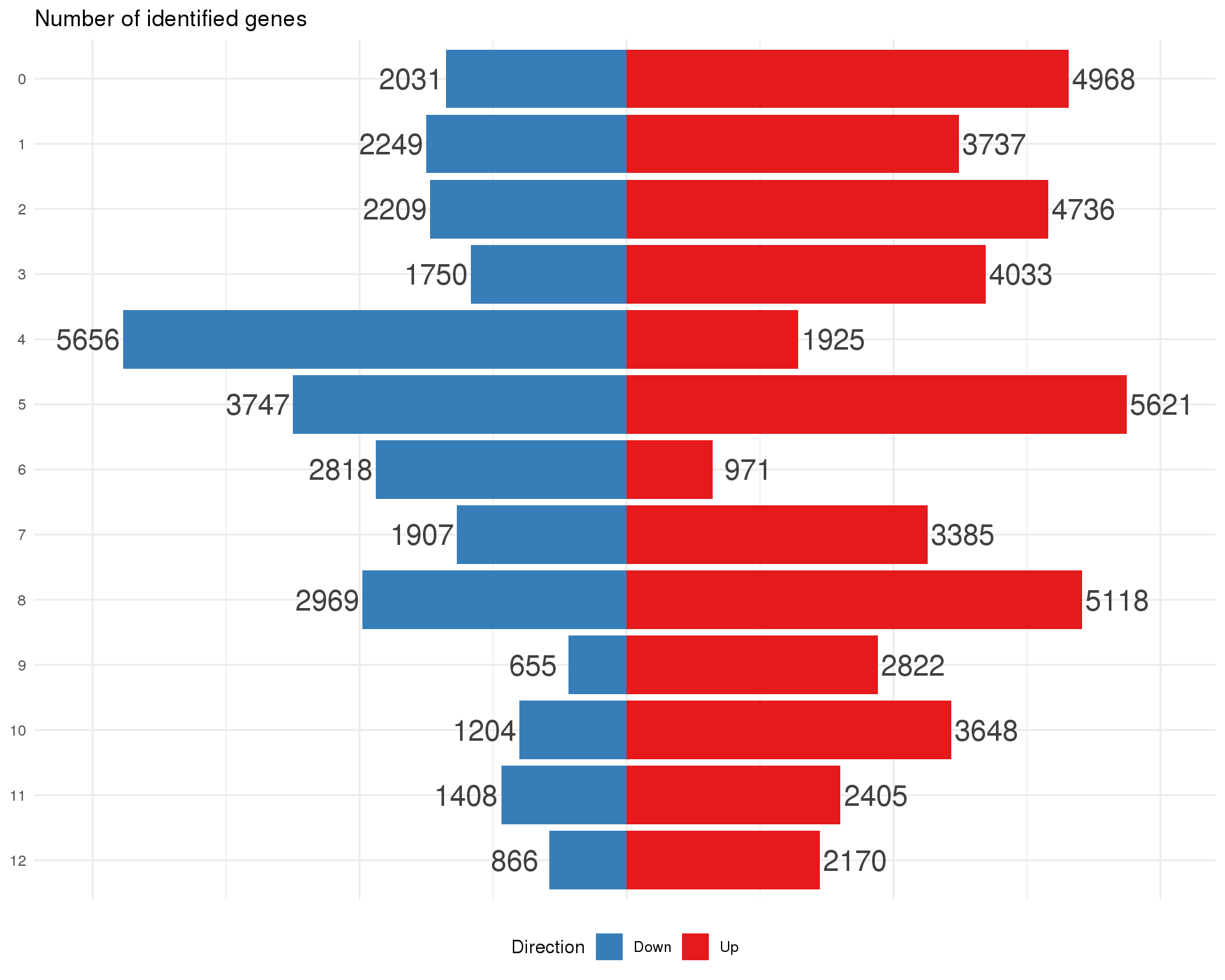
Table
Table of significant genes for each cluster with log fold-change greater than one.
src_list <- lapply(seq_len(n_clusts) - 1, function(clust) {
    src <- c(
        "### Cluster {{clust}} {.unnumbered}",
        "```{r table-{{clust}}}",
        "markers_list[[{{clust}} + 1]]",
        "```",
        ""
    )
    knit_expand(text = src)
})

out <- knit_child(text = unlist(src_list), options = list(cache = FALSE))
Cluster 0
markers_list[[0 + 1]]Cluster 1
markers_list[[1 + 1]]Cluster 2
markers_list[[2 + 1]]Cluster 3
markers_list[[3 + 1]]Cluster 4
markers_list[[4 + 1]]Cluster 5
markers_list[[5 + 1]]Cluster 6
markers_list[[6 + 1]]Cluster 7
markers_list[[7 + 1]]Cluster 8
markers_list[[8 + 1]]Cluster 9
markers_list[[9 + 1]]Cluster 10
markers_list[[10 + 1]]Cluster 11
markers_list[[11 + 1]]Cluster 12
markers_list[[12 + 1]]Known genes
To help with identifying clusters we will look at some previously identified marker genes.
known_genes <- c(
    # Stroma
    "TAGLN", "ACTA2", "MAB21L2", "DLK1", "GATA3", "COL2A1", "COL9A3",
    # Podocyte
    "PODXL", "NPHS2", "TCF21",
    # Cell cycle
    "HIST1H4C", "PCLAF", "CENPF", "HMGB2",
    # Endothelium
    "CLDN5", "PECAM1", "KDR", "CALM1",
    # Neural
    "TTYH1", "SOX2", "HES6", "STMN2",
    # Epithelium
    "PAX2", "PAX8", "KRT19",
    # Muscle
    "MYOG", "MYOD1",
    # Immune
    "TYROBP", "MPO", "S100A9"
)

known_types <- factor(c(
    rep("Stroma", 7),
    rep("Podocyte", 3),
    rep("Cell cycle", 4),
    rep("Endothelium", 4),
    rep("Neural", 4),
    rep("Epithelium", 3),
    rep("Muscle", 2),
    rep("Immune", 3)
))
names(known_types) <- known_genes
Expression
Size indicates (scaled) mean expression level, transparency indicate proportion of cells expressing the gene.
plot_data <- map_df(seq_len(n_clusts), function(idx) {
    clust_cells <- colData(sce_filt)$Cluster == idx - 1
    means <- Matrix::rowMeans(logcounts(sce_filt)[known_genes, clust_cells])
    props <- Matrix::rowSums(counts(sce_filt)[known_genes, clust_cells] > 0) /
                                 sum(clust_cells)
    tibble(Cluster = idx - 1,
           Gene = known_genes,
           Type = known_types,
           Mean = means,
           Prop = props)
}) %>%
    mutate(Cluster = factor(Cluster, levels = (n_clusts - 1):0),
           Gene = factor(Gene, levels = known_genes),
           Type = factor(Type, levels = unique(known_types))) %>%
    group_by(Gene) %>%
    mutate(Mean = scale(Mean))

ggplot(plot_data,
       aes(x = Gene, y = Cluster, size = Prop, alpha = Mean, colour = Type)) +
    geom_point() +
    guides(size = FALSE, alpha = FALSE) +
    facet_grid(~ Type, scales = "free_x", space = "free_x") +
    theme_minimal() +
    theme(axis.title.x = element_blank(),
          axis.text.x = element_text(angle = 90, hjust = 1, vjust = 0.5),
          legend.position = "none")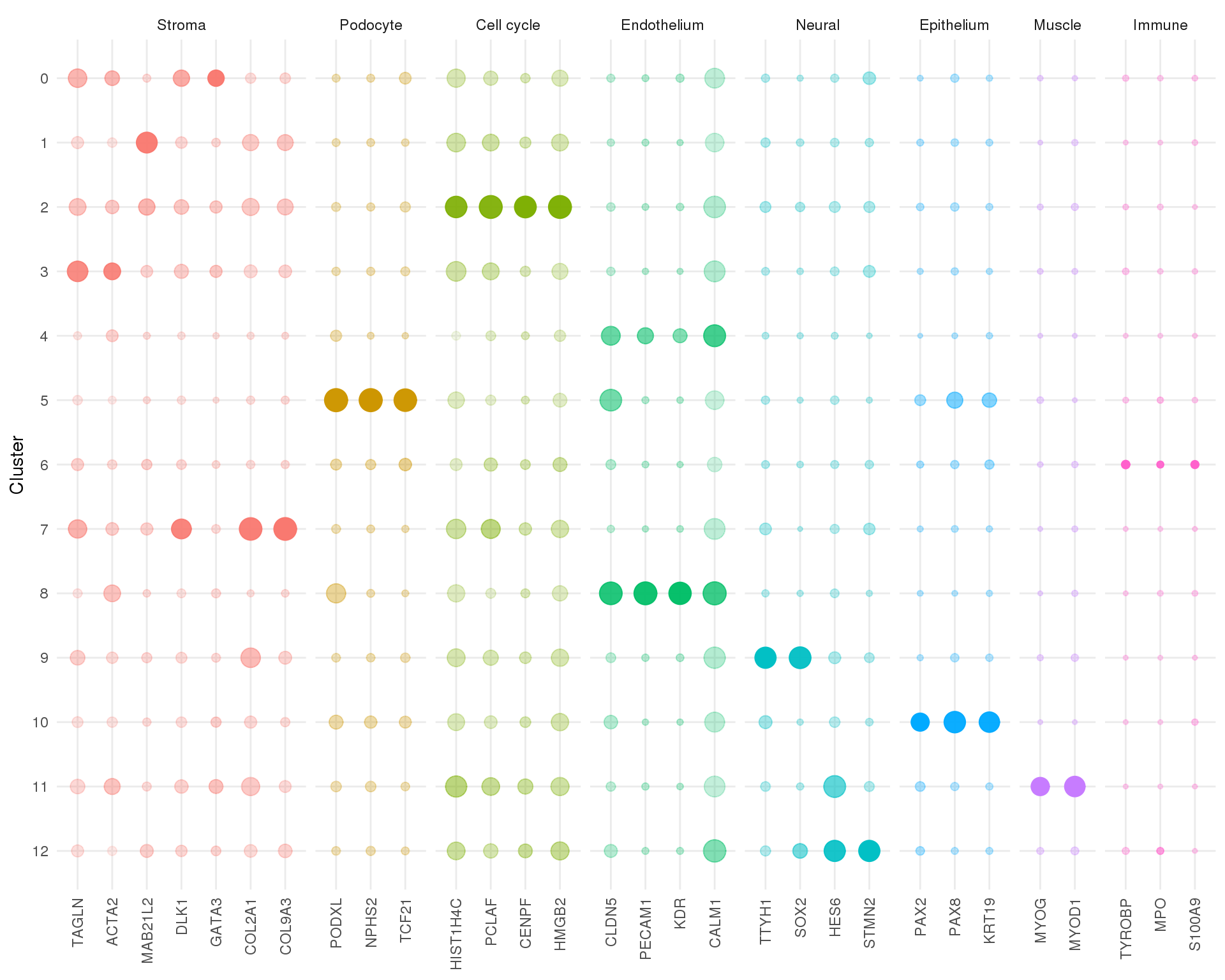
Significance
Size indicates log fold-change and transparency indicates significance. As we are only interested in marker genes negative fold-changes have been set to zero and significance for those cases has been set to one.
plot_data <- map_df(seq_len(n_clusts), function(idx) {
    de_list[[idx]] %>%
        filter(Name %in% known_genes)
}) %>%
    mutate(FDR = if_else(logFC < 0, 1, FDR)) %>%
    mutate(logFC = if_else(logFC < 0, 0, logFC)) %>%
    mutate(Type = known_types[Name]) %>%
    mutate(Cluster = factor(Cluster, levels = (n_clusts - 1):0),
           Gene = factor(Name, levels = known_genes),
           Type = factor(Type, levels = unique(known_types)))

ggplot(plot_data,
       aes(x = Gene, y = Cluster, size = logFC, alpha = -FDR, colour = Type)) +
    geom_point() +
    facet_grid(~ Type, scales = "free_x", space = "free_x") +
    theme_minimal() +
    theme(axis.title.x = element_blank(),
          axis.text.x = element_text(angle = 90, hjust = 1, vjust = 0.5),
          legend.position = "none")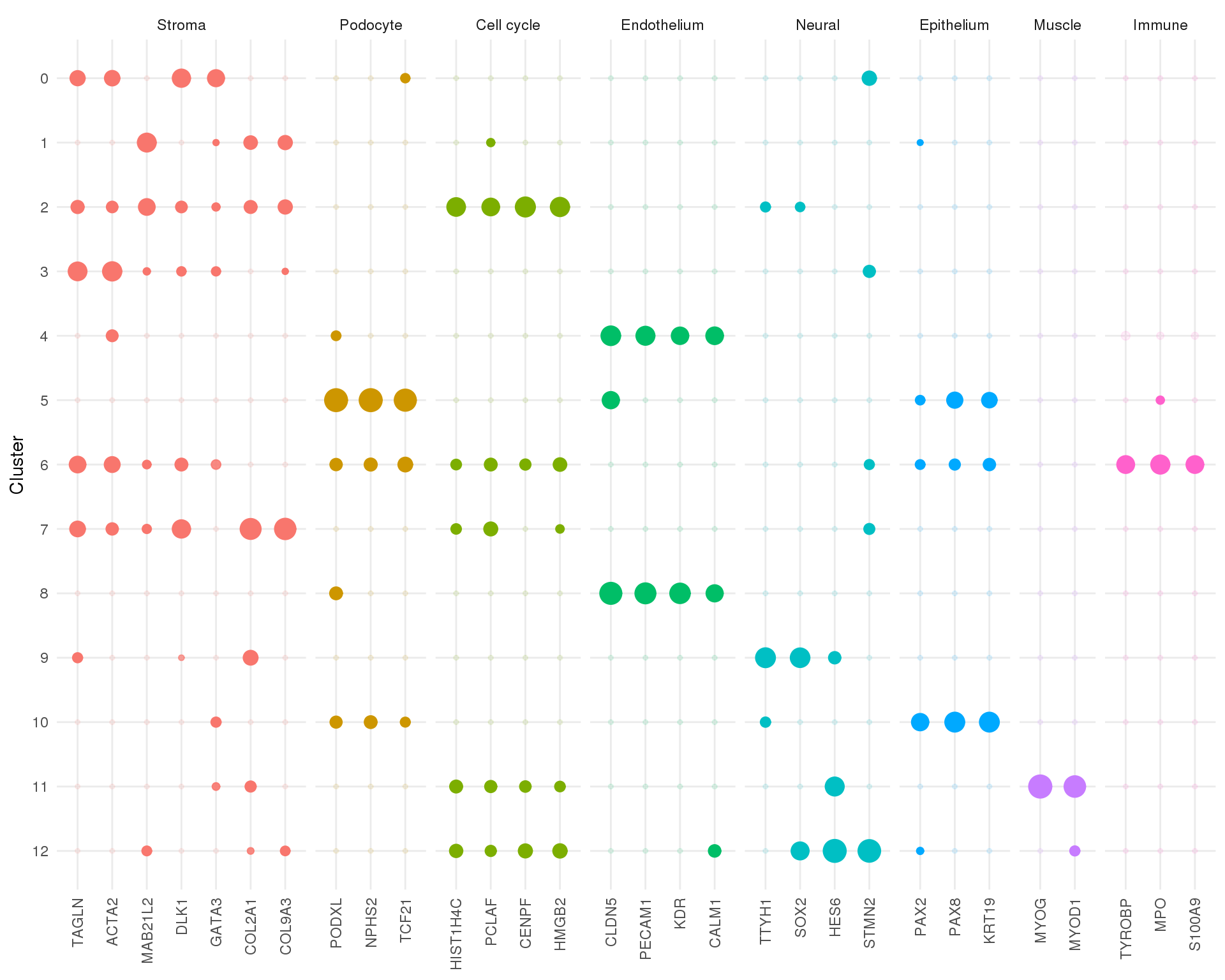
Figures
plot_data <- tibble(Observed = log1p(Matrix::rowMeans(counts(sce_filt))),
                    Expected = log1p(rowMeans(de_fit$fitted.values))) %>%
    mutate(Mean = 0.5 * (Observed + Expected),
           Difference = Observed - Expected)

mean_plot <- ggplot(plot_data, aes(x = Mean, y = Difference)) +
    geom_point(alpha = 0.3, colour = "#7A52C7") +
    geom_smooth(method = "loess", colour = "#00ADEF",
                fill = "#00ADEF", size = 1) +
    geom_hline(yintercept = 0, colour = "#EC008C", size = 1) +
    xlab("0.5 * (Observed mean + Expected mean)") +
    ylab("Observed mean - Expected mean") +
    ggtitle("Fit of gene means") +
    theme_minimal()

plot_data <- tibble(Observed = Matrix::rowMeans(counts(sce_filt) == 0),
                    Expected = rowMeans(
                        (1 + de_fit$fitted.values * dge$tagwise.dispersion) ^
                            (-1 / dge$tagwise.dispersion)
                    )) %>%
    mutate(Mean = 0.5 * (Observed + Expected),
           Difference = Observed - Expected)

zeros_plot <- ggplot(plot_data, aes(x = Mean, y = Difference)) +
    geom_point(alpha = 0.3, colour = "#7A52C7") +
    geom_smooth(method = "loess", colour = "#00ADEF",
                fill = "#00ADEF", size = 1) +
    geom_hline(yintercept = 0, colour = "#EC008C", size = 1) +
    xlab("0.5 * (Observed proportion zeros + Expected proportion zeros)") +
    ylab("Observed proportion zeros - Expected proportion zeros") +
    ggtitle("Fit of gene proportion of zeros") +
    theme_minimal()

plot_data <- tibble(
    AvgLogCPM = dge$AveLogCPM,
    Tagwise = dge$tagwise.dispersion,
    Trended = dge$trended.dispersion
)

bcv_plot <- ggplot(plot_data, aes(x = AvgLogCPM)) +
    geom_point(aes(y = sqrt(Tagwise)), alpha = 0.3, colour = "#7A52C7") +
    geom_hline(yintercept = sqrt(dge$common.dispersion),
               colour = "#EC008C", size = 1) +
    geom_line(aes(y = sqrt(Trended)), colour = "#00ADEF", size = 1) +
    ggtitle("edgeR biological coefficient of variation") +
    xlab(expression("Average counts per million ("*log["2"]*")")) +
    ylab("Biological coefficient of variation") +
    theme_minimal()

plot_data <- de_list %>%
    bind_rows() %>%
    filter(FDR < 0.05) %>%
    mutate(IsUp = logFC > 0) %>%
    filter(IsUp) %>%
    mutate(MaxLogFC = max(logFC)) %>%
    group_by(Cluster) %>%
    mutate(logFCScaled = scales::rescale(
        logFC, from = c(0, max(MaxLogFC)), to = c(0, n()))
    ) %>%
    ungroup() %>%
    mutate(Cluster = factor(Cluster, levels = 0:(n_clusts - 1)))

counts_plot <- ggplot(plot_data, aes(x = Cluster)) +
    geom_bar(aes(fill = Cluster), alpha = 0.3) +
    geom_jitter(aes(y = logFCScaled, colour = logFC),
                position = position_jitter(height = 0, width = 0.35, seed = 1),
                alpha = 0.3) +
    geom_text(aes(label=..count..), stat = "count",
              vjust = -0.5, size = 4, colour = "grey10") +
    scale_fill_discrete(guide = FALSE) +
    scale_colour_viridis_c(option = "plasma") +
    ggtitle("Up-regulated DE genes by cluster") +
    theme_minimal() +
    theme(plot.title = element_text(size = rel(1.2), hjust = 0.1,
                                    vjust = 1, margin = margin(1)),
          axis.title = element_blank(),
          axis.text.y = element_blank(),
          panel.grid = element_blank())

plot_data <- map_df(seq_len(n_clusts), function(idx) {
    de_list[[idx]] %>%
        filter(Name %in% known_genes)
}) %>%
    mutate(FDR = if_else(logFC < 0, 1, FDR)) %>%
    mutate(logFC = if_else(logFC < 0, 0, logFC)) %>%
    mutate(Type = known_types[Name]) %>%
    mutate(Cluster = factor(Cluster, levels = (n_clusts - 1):0),
           Gene = factor(Name, levels = known_genes),
           Type = factor(Type, levels = unique(known_types)))

genes_plot <- ggplot(plot_data,
       aes(x = Gene, y = Cluster, size = logFC, alpha = -FDR, colour = Type)) +
    geom_point() +
    facet_grid(~ Type, scales = "free_x", space = "free_x") +
    ggtitle("edgeR results for some published markers by cluster") +
    theme_minimal() +
    theme(axis.title = element_blank(),
          axis.text.x = element_text(angle = 90, hjust = 1, vjust = 0.5),
          legend.position = "none")

p1 <- plot_grid(mean_plot, zeros_plot, bcv_plot, counts_plot,
                ncol = 2, labels = "AUTO")

fig <- plot_grid(p1, genes_plot, ncol = 1, labels = c("", "E"),
                 rel_heights = c(1, 0.5))

ggsave(here::here("output", DOCNAME, "de-results.pdf"), fig,
       width = 7, height = 10, scale = 1.5)
ggsave(here::here("output", DOCNAME, "de-results.png"), fig,
       width = 7, height = 10, scale = 1.5)

fig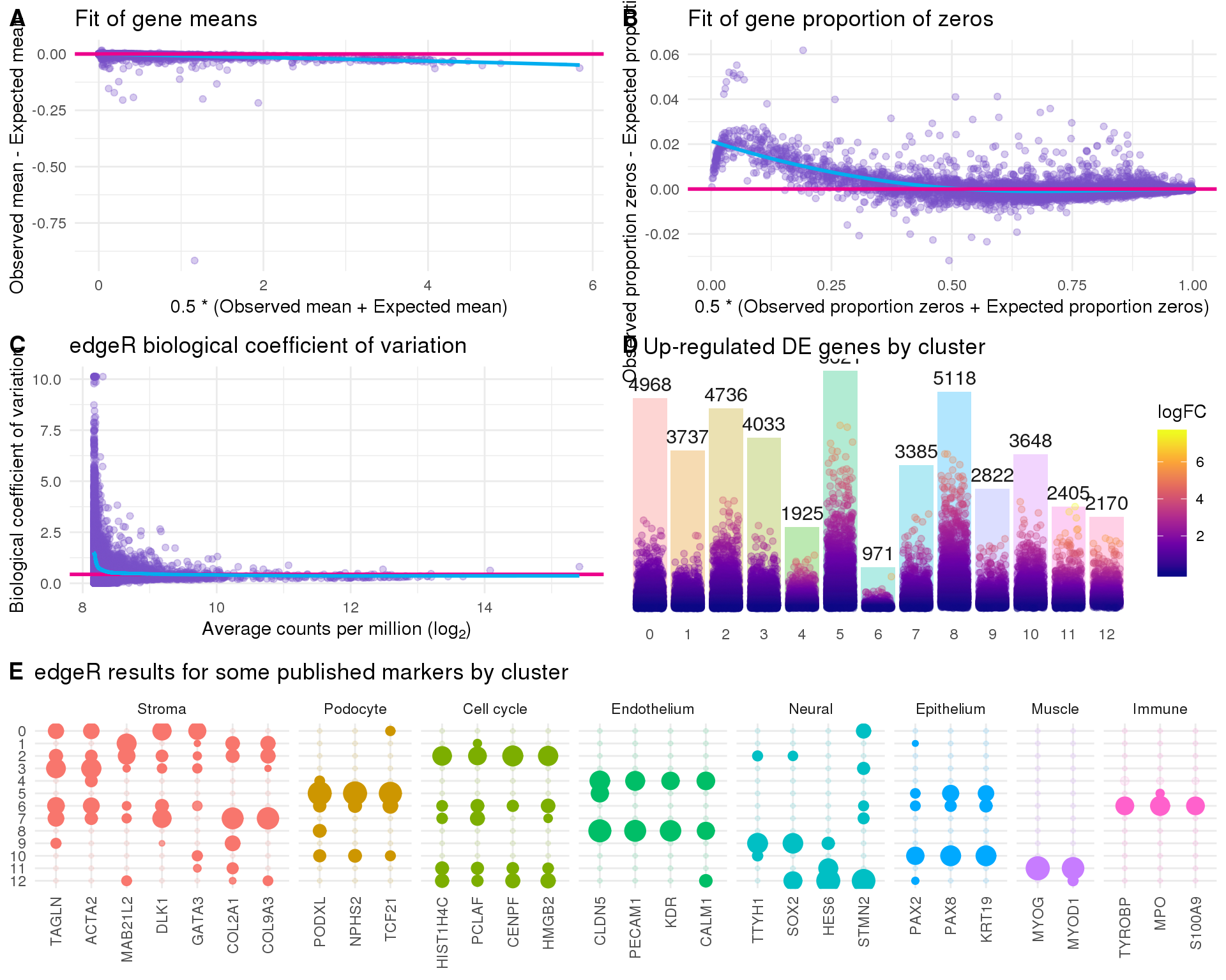
Summary
Based on the detected markers we will assign the following cell types to the clusters.
assignments <- tribble(
    ~Cluster,         ~Assignment,
         "0",            "Stroma",
         "1",            "Stroma",
         "2",        "Cell cycle",
         "3",            "Stroma",
         "4",       "Endothelium",
         "5",          "Podocyte",
         "6",   "Possible immune",
         "7",            "Stroma",
         "8",       "Endothelium",
         "9",             "Glial",
        "10",        "Epithelium",
        "11", "Muscle progenitor",
        "12", "Neural progenitor"
)

assignments
Parameters
This table describes parameters used and set in this document.
params <- list(
    list(
        Parameter = "maxmean_thresh",
        Value = maxmean_thresh,
        Description = "Minimum threshold for (log10) maxium cluster mean"
    ),
    list(
        Parameter = "maxmean_mads",
        Value = maxmean_mads,
        Description = "MADs for (log10) maxium cluster mean"
    ),
    list(
        Parameter = "fdr_thresh",
        Value = fdr_thresh,
        Description = "FDR threshold for significant marker genes"
    ),
    list(
        Parameter = "logFC_thresh",
        Value = logFC_thresh,
        Description = "Log foldchange threshold for significant marker genes"
    )
)

params <- jsonlite::toJSON(params, pretty = TRUE)
knitr::kable(jsonlite::fromJSON(params))| Parameter | Value | Description |
|---|---|---|
| maxmean_thresh | -1.3505 | Minimum threshold for (log10) maxium cluster mean |
| maxmean_mads | 0.5 | MADs for (log10) maxium cluster mean |
| fdr_thresh | 0.05 | FDR threshold for significant marker genes |
| logFC_thresh | 1 | Log foldchange threshold for significant marker genes |
Output files
This table describes the output files produced by this document. Right click and Save Link As… to download the results.
write_rds(sce, here::here("data/processed/04-markers.Rds"))
write_rds(de_fit, here::here("data/processed/04-DGEGLM.Rds"))
dir.create(here::here("output", DOCNAME), showWarnings = FALSE)
readr::write_lines(params, here::here("output", DOCNAME, "parameters.json"))
writeGeneTable(de_list, here::here("output", DOCNAME, "de_genes.xlsx"))
writeGeneTable(bind_rows(de_list),
here::here("output", DOCNAME, "de_genes.csv"))
readr::write_tsv(assignments, here::here("output", DOCNAME, "assignments.tsv"))
knitr::kable(data.frame(
File = c(
getDownloadLink("parameters.json", DOCNAME),
getDownloadLink("de_genes.xlsx", DOCNAME),
getDownloadLink("de_genes.csv.zip", DOCNAME),
getDownloadLink("assignments.csv", DOCNAME),
getDownloadLink("de-results.png", DOCNAME),
getDownloadLink("de-results.pdf", DOCNAME)
),
Description = c(
"Parameters set and used in this analysis",
paste("Results of marker gene testing in XLSX format with one tab",
"per cluster"),
"Results of marker gene testing in zipped CSV format",
"Cluster assignments (TSV)",
"DE results figure (PNG)",
"DE results figure (PDF)"
)
))| File | Description |
|---|---|
| parameters.json | Parameters set and used in this analysis |
| de_genes.xlsx | Results of marker gene testing in XLSX format with one tab per cluster |
| de_genes.csv.zip | Results of marker gene testing in zipped CSV format |
| assignments.csv | Cluster assignments (TSV) |
| de-results.png | DE results figure (PNG) |
| de-results.pdf | DE results figure (PDF) |
Session information
devtools::session_info()─ Session info ──────────────────────────────────────────────────────────
setting value
version R version 3.5.0 (2018-04-23)
os CentOS release 6.7 (Final)
system x86_64, linux-gnu
ui X11
language (EN)
collate en_US.UTF-8
ctype en_US.UTF-8
tz Australia/Melbourne
date 2019-04-03
─ Packages ──────────────────────────────────────────────────────────────
! package * version date lib source
assertthat 0.2.0 2017-04-11 [1] CRAN (R 3.5.0)
backports 1.1.3 2018-12-14 [1] CRAN (R 3.5.0)
beeswarm 0.2.3 2016-04-25 [1] CRAN (R 3.5.0)
bindr 0.1.1 2018-03-13 [1] CRAN (R 3.5.0)
bindrcpp 0.2.2 2018-03-29 [1] CRAN (R 3.5.0)
Biobase * 2.42.0 2018-10-30 [1] Bioconductor
BiocGenerics * 0.28.0 2018-10-30 [1] Bioconductor
BiocParallel * 1.16.5 2019-01-04 [1] Bioconductor
bitops 1.0-6 2013-08-17 [1] CRAN (R 3.5.0)
broom 0.5.1 2018-12-05 [1] CRAN (R 3.5.0)
callr 3.1.1 2018-12-21 [1] CRAN (R 3.5.0)
cellranger 1.1.0 2016-07-27 [1] CRAN (R 3.5.0)
cli 1.0.1 2018-09-25 [1] CRAN (R 3.5.0)
colorspace 1.4-0 2019-01-13 [1] CRAN (R 3.5.0)
cowplot * 0.9.4 2019-01-08 [1] CRAN (R 3.5.0)
crayon 1.3.4 2017-09-16 [1] CRAN (R 3.5.0)
DelayedArray * 0.8.0 2018-10-30 [1] Bioconductor
DelayedMatrixStats 1.4.0 2018-10-30 [1] Bioconductor
desc 1.2.0 2018-05-01 [1] CRAN (R 3.5.0)
devtools 2.0.1 2018-10-26 [1] CRAN (R 3.5.0)
digest 0.6.18 2018-10-10 [1] CRAN (R 3.5.0)
dplyr * 0.7.8 2018-11-10 [1] CRAN (R 3.5.0)
edgeR * 3.24.3 2019-01-02 [1] Bioconductor
evaluate 0.12 2018-10-09 [1] CRAN (R 3.5.0)
forcats * 0.3.0 2018-02-19 [1] CRAN (R 3.5.0)
fs 1.2.6 2018-08-23 [1] CRAN (R 3.5.0)
generics 0.0.2 2018-11-29 [1] CRAN (R 3.5.0)
GenomeInfoDb * 1.18.1 2018-11-12 [1] Bioconductor
GenomeInfoDbData 1.2.0 2019-01-15 [1] Bioconductor
GenomicRanges * 1.34.0 2018-10-30 [1] Bioconductor
ggbeeswarm 0.6.0 2017-08-07 [1] CRAN (R 3.5.0)
ggplot2 * 3.1.0 2018-10-25 [1] CRAN (R 3.5.0)
git2r 0.24.0 2019-01-07 [1] CRAN (R 3.5.0)
glue 1.3.0 2018-07-17 [1] CRAN (R 3.5.0)
gridExtra 2.3 2017-09-09 [1] CRAN (R 3.5.0)
gtable 0.2.0 2016-02-26 [1] CRAN (R 3.5.0)
haven 2.0.0 2018-11-22 [1] CRAN (R 3.5.0)
HDF5Array 1.10.1 2018-12-05 [1] Bioconductor
here 0.1 2017-05-28 [1] CRAN (R 3.5.0)
hms 0.4.2 2018-03-10 [1] CRAN (R 3.5.0)
htmltools 0.3.6 2017-04-28 [1] CRAN (R 3.5.0)
httr 1.4.0 2018-12-11 [1] CRAN (R 3.5.0)
IRanges * 2.16.0 2018-10-30 [1] Bioconductor
jsonlite 1.6 2018-12-07 [1] CRAN (R 3.5.0)
knitr * 1.21 2018-12-10 [1] CRAN (R 3.5.0)
P lattice 0.20-35 2017-03-25 [5] CRAN (R 3.5.0)
lazyeval 0.2.1 2017-10-29 [1] CRAN (R 3.5.0)
limma * 3.38.3 2018-12-02 [1] Bioconductor
locfit 1.5-9.1 2013-04-20 [1] CRAN (R 3.5.0)
lubridate 1.7.4 2018-04-11 [1] CRAN (R 3.5.0)
magrittr 1.5 2014-11-22 [1] CRAN (R 3.5.0)
P Matrix 1.2-14 2018-04-09 [5] CRAN (R 3.5.0)
matrixStats * 0.54.0 2018-07-23 [1] CRAN (R 3.5.0)
memoise 1.1.0 2017-04-21 [1] CRAN (R 3.5.0)
modelr 0.1.3 2019-02-05 [1] CRAN (R 3.5.0)
munsell 0.5.0 2018-06-12 [1] CRAN (R 3.5.0)
P nlme 3.1-137 2018-04-07 [5] CRAN (R 3.5.0)
pillar 1.3.1 2018-12-15 [1] CRAN (R 3.5.0)
pkgbuild 1.0.2 2018-10-16 [1] CRAN (R 3.5.0)
pkgconfig 2.0.2 2018-08-16 [1] CRAN (R 3.5.0)
pkgload 1.0.2 2018-10-29 [1] CRAN (R 3.5.0)
plyr 1.8.4 2016-06-08 [1] CRAN (R 3.5.0)
prettyunits 1.0.2 2015-07-13 [1] CRAN (R 3.5.0)
processx 3.2.1 2018-12-05 [1] CRAN (R 3.5.0)
ps 1.3.0 2018-12-21 [1] CRAN (R 3.5.0)
purrr * 0.3.0 2019-01-27 [1] CRAN (R 3.5.0)
R.methodsS3 1.7.1 2016-02-16 [1] CRAN (R 3.5.0)
R.oo 1.22.0 2018-04-22 [1] CRAN (R 3.5.0)
R.utils 2.7.0 2018-08-27 [1] CRAN (R 3.5.0)
R6 2.3.0 2018-10-04 [1] CRAN (R 3.5.0)
Rcpp 1.0.0 2018-11-07 [1] CRAN (R 3.5.0)
RCurl 1.95-4.11 2018-07-15 [1] CRAN (R 3.5.0)
readr * 1.3.1 2018-12-21 [1] CRAN (R 3.5.0)
readxl 1.2.0 2018-12-19 [1] CRAN (R 3.5.0)
remotes 2.0.2 2018-10-30 [1] CRAN (R 3.5.0)
reshape2 1.4.3 2017-12-11 [1] CRAN (R 3.5.0)
rhdf5 2.26.2 2019-01-02 [1] Bioconductor
Rhdf5lib 1.4.2 2018-12-03 [1] Bioconductor
rlang 0.3.1 2019-01-08 [1] CRAN (R 3.5.0)
rmarkdown 1.11 2018-12-08 [1] CRAN (R 3.5.0)
rprojroot 1.3-2 2018-01-03 [1] CRAN (R 3.5.0)
rstudioapi 0.9.0 2019-01-09 [1] CRAN (R 3.5.0)
rvest 0.3.2 2016-06-17 [1] CRAN (R 3.5.0)
S4Vectors * 0.20.1 2018-11-09 [1] Bioconductor
scales 1.0.0 2018-08-09 [1] CRAN (R 3.5.0)
scater * 1.10.1 2019-01-04 [1] Bioconductor
sessioninfo 1.1.1 2018-11-05 [1] CRAN (R 3.5.0)
SingleCellExperiment * 1.4.1 2019-01-04 [1] Bioconductor
stringi 1.2.4 2018-07-20 [1] CRAN (R 3.5.0)
stringr * 1.3.1 2018-05-10 [1] CRAN (R 3.5.0)
SummarizedExperiment * 1.12.0 2018-10-30 [1] Bioconductor
testthat 2.0.1 2018-10-13 [4] CRAN (R 3.5.0)
tibble * 2.0.1 2019-01-12 [1] CRAN (R 3.5.0)
tidyr * 0.8.2 2018-10-28 [1] CRAN (R 3.5.0)
tidyselect 0.2.5 2018-10-11 [1] CRAN (R 3.5.0)
tidyverse * 1.2.1 2017-11-14 [1] CRAN (R 3.5.0)
usethis 1.4.0 2018-08-14 [1] CRAN (R 3.5.0)
vipor 0.4.5 2017-03-22 [1] CRAN (R 3.5.0)
viridis 0.5.1 2018-03-29 [1] CRAN (R 3.5.0)
viridisLite 0.3.0 2018-02-01 [1] CRAN (R 3.5.0)
whisker 0.3-2 2013-04-28 [1] CRAN (R 3.5.0)
withr 2.1.2 2018-03-15 [1] CRAN (R 3.5.0)
workflowr 1.1.1 2018-07-06 [1] CRAN (R 3.5.0)
xfun 0.4 2018-10-23 [1] CRAN (R 3.5.0)
xml2 1.2.0 2018-01-24 [1] CRAN (R 3.5.0)
XVector 0.22.0 2018-10-30 [1] Bioconductor
yaml 2.2.0 2018-07-25 [1] CRAN (R 3.5.0)
zlibbioc 1.28.0 2018-10-30 [1] Bioconductor
[1] /group/bioi1/luke/analysis/phd-thesis-analysis/packrat/lib/x86_64-pc-linux-gnu/3.5.0
[2] /group/bioi1/luke/analysis/phd-thesis-analysis/packrat/lib-ext/x86_64-pc-linux-gnu/3.5.0
[3] /group/bioi1/luke/analysis/phd-thesis-analysis/packrat/lib-R/x86_64-pc-linux-gnu/3.5.0
[4] /home/luke.zappia/R/x86_64-pc-linux-gnu-library/3.5
[5] /usr/local/installed/R/3.5.0/lib64/R/library
P ── Loaded and on-disk path mismatch.This reproducible R Markdown analysis was created with workflowr 1.1.1