Pre-processing
Last updated: 2019-04-03
workflowr checks: (Click a bullet for more information)-
✔ R Markdown file: up-to-date
Great! Since the R Markdown file has been committed to the Git repository, you know the exact version of the code that produced these results.
-
✔ Environment: empty
Great job! The global environment was empty. Objects defined in the global environment can affect the analysis in your R Markdown file in unknown ways. For reproduciblity it’s best to always run the code in an empty environment.
-
✔ Seed:
set.seed(20190110)The command
set.seed(20190110)was run prior to running the code in the R Markdown file. Setting a seed ensures that any results that rely on randomness, e.g. subsampling or permutations, are reproducible. -
✔ Session information: recorded
Great job! Recording the operating system, R version, and package versions is critical for reproducibility.
-
Great! You are using Git for version control. Tracking code development and connecting the code version to the results is critical for reproducibility. The version displayed above was the version of the Git repository at the time these results were generated.✔ Repository version: 5870e6e
Note that you need to be careful to ensure that all relevant files for the analysis have been committed to Git prior to generating the results (you can usewflow_publishorwflow_git_commit). workflowr only checks the R Markdown file, but you know if there are other scripts or data files that it depends on. Below is the status of the Git repository when the results were generated:
Note that any generated files, e.g. HTML, png, CSS, etc., are not included in this status report because it is ok for generated content to have uncommitted changes.Ignored files: Ignored: .DS_Store Ignored: .Rhistory Ignored: .Rproj.user/ Ignored: ._.DS_Store Ignored: analysis/cache/ Ignored: build-logs/ Ignored: data/alevin/ Ignored: data/cellranger/ Ignored: data/processed/ Ignored: data/published/ Ignored: output/.DS_Store Ignored: output/._.DS_Store Ignored: output/03-clustering/selected_genes.csv.zip Ignored: output/04-marker-genes/de_genes.csv.zip Ignored: packrat/.DS_Store Ignored: packrat/._.DS_Store Ignored: packrat/lib-R/ Ignored: packrat/lib-ext/ Ignored: packrat/lib/ Ignored: packrat/src/ Untracked files: Untracked: DGEList.Rds Untracked: output/90-methods/package-versions.json Untracked: scripts/build.pbs Unstaged changes: Modified: analysis/_site.yml Modified: output/01-preprocessing/droplet-selection.pdf Modified: output/01-preprocessing/parameters.json Modified: output/01-preprocessing/selection-comparison.pdf Modified: output/01B-alevin/alevin-comparison.pdf Modified: output/01B-alevin/parameters.json Modified: output/02-quality-control/qc-thresholds.pdf Modified: output/02-quality-control/qc-validation.pdf Modified: output/03-clustering/cluster-comparison.pdf Modified: output/03-clustering/cluster-validation.pdf Modified: output/04-marker-genes/de-results.pdf
Expand here to see past versions:
| File | Version | Author | Date | Message |
|---|---|---|---|---|
| Rmd | 5870e6e | Luke Zappia | 2019-04-03 | Adjust figures and fix names |
| html | 33ac14f | Luke Zappia | 2019-03-20 | Tidy up website |
| Rmd | ae75188 | Luke Zappia | 2019-03-06 | Revise figures after proofread |
| html | ae75188 | Luke Zappia | 2019-03-06 | Revise figures after proofread |
| html | 2693e97 | Luke Zappia | 2019-03-05 | Add methods page |
| html | 4a2f376 | Luke Zappia | 2019-02-20 | Add default Cell Ranger and update figures |
| Rmd | 431c180 | Luke Zappia | 2019-02-19 | Add droplet selection figure |
| html | 431c180 | Luke Zappia | 2019-02-19 | Add droplet selection figure |
| Rmd | 8f826ef | Luke Zappia | 2019-02-08 | Rebuild site and tidy |
| html | 8f826ef | Luke Zappia | 2019-02-08 | Rebuild site and tidy |
| Rmd | 2daa7f2 | Luke Zappia | 2019-01-25 | Improve output and rebuild |
| html | 2daa7f2 | Luke Zappia | 2019-01-25 | Improve output and rebuild |
| Rmd | b4432ff | Luke Zappia | 2019-01-18 | Add emptyDrops p-value plot |
| html | b4432ff | Luke Zappia | 2019-01-18 | Add emptyDrops p-value plot |
| html | bf40049 | Luke Zappia | 2019-01-18 | Add preprocessing |
# scRNA-seq
library("DropletUtils")
library("SingleCellExperiment")

# Plotting
library("cowplot")
library("UpSetR")
library("grid")

# Tidyverse
library("tidyverse")
source(here::here("R/load.R"))
source(here::here("R/annotate.R"))
source(here::here("R/output.R"))bpparam <- BiocParallel::MulticoreParam(workers = 10)Introduction
In this document we are going to read in the unfiltered counts matrix produced by Cell Ranger and determine which of those droplets contain cells using the DropletUtils package.
path <- here::here("data/cellranger")
raw <- read10x(path, dataset = "Orgs123")

filt_barcodes <- readr::read_lines(file.path(path, "filtered_barcodes.tsv.gz"))

colData(raw)$CellRangerFilt <- paste(colData(raw)$Barcode,
                                     colData(raw)$Sample, sep = "-") %in%
    filt_barcodes
The raw dataset has 33538 features and 2211840 droplets.
raw <- raw[Matrix::rowSums(counts(raw)) > 0, Matrix::colSums(counts(raw)) > 0]After removing all zero features and droplets the dataset has 25020 features and 945038 droplets.
Barcode ranks
empty_thresh <- 100

bc_ranks <- barcodeRanks(counts(raw), lower = empty_thresh)

colData(raw)$BarcodeRank   <- bc_ranks$rank
colData(raw)$BarcodeTotal  <- bc_ranks$total
colData(raw)$BarcodeFitted <- bc_ranks$fitted

bc_data <- colData(raw) %>%
    as.data.frame() %>%
    select(Cell, Kept = CellRangerFilt, Rank = BarcodeRank,
           Total = BarcodeTotal, Fitted = BarcodeFitted) %>%
    arrange(Rank)
Let’s start by ordering the droplets according to their total counts and plotting this on a log scale. This let’s us see the distribution of total counts.
ggplot(bc_data, aes(x = Rank, y = Total)) +
    geom_point(shape = 1, aes(colour = Kept)) +
    geom_line(aes(y = Fitted), colour = "red") +
    geom_hline(yintercept = bc_ranks$knee,
               colour = "dodgerblue", linetype = "dashed") +
    annotate("text", x = 0, y = bc_ranks$knee, label = "Knee",
             colour = "dodgerblue", hjust = 0, vjust = -1) +
    geom_hline(yintercept = bc_ranks$inflection,
               colour = "forestgreen", linetype = "dashed") +
    annotate("text", x = 0, y = bc_ranks$inflection, label = "Inflection",
             colour = "forestgreen", hjust = 0, vjust = -1) +
    geom_hline(yintercept = empty_thresh,
               colour = "darkorchid", linetype = "dashed") +
    annotate("text", x = 0, y = empty_thresh, label = "Empty threshold",
             colour = "darkorchid", hjust = 0, vjust = -1) +
    scale_x_log10(labels = scales::number) +
    scale_y_log10(labels = scales::number) +
    scale_colour_manual(values = c("black", "violet")) +
    ylab("Total counts") +
    theme_minimal()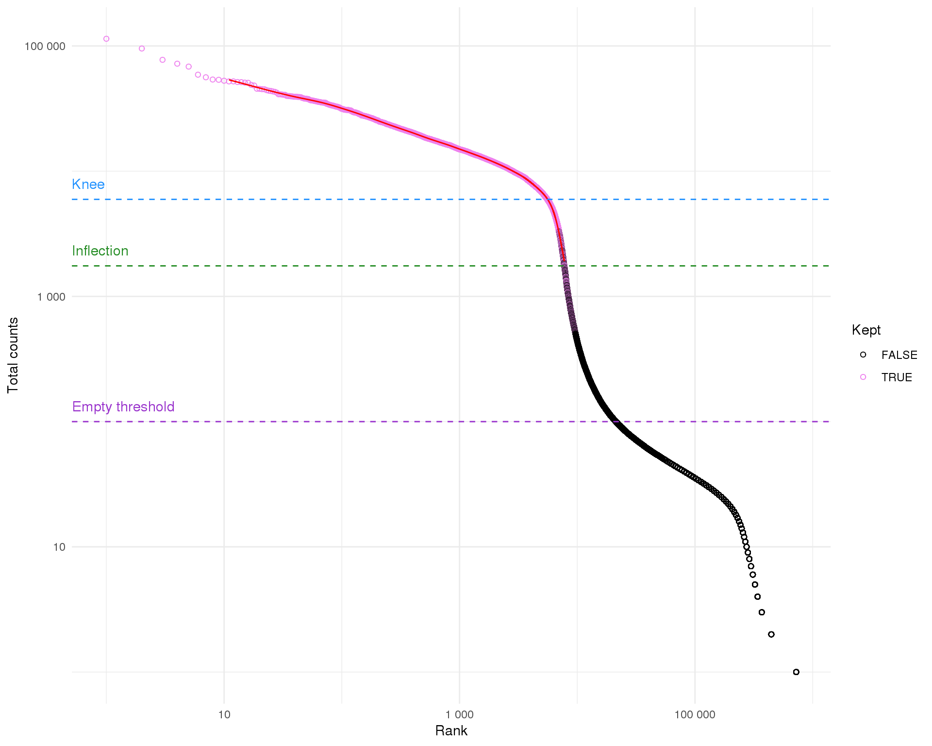
Expand here to see past versions of barcodes-plot-1.png:
| Version | Author | Date |
|---|---|---|
| bf40049 | Luke Zappia | 2019-01-18 |
This is typical of what we see for 10x experiment where there is a sharp drop off between droplets with lots of counts and those without many. The inflection and knee points are methods for identifying the transition between distributions. These are roughly associated with the cells selected by Cell Ranger The empty threshold line indicates the point at which we assume droplets must be empty (total counts <= 100).
Traditional Cell Ranger
The version of Cell Ranger we have used here selects cells using a modified version of the EmptyDrops method (see below) but older versions used an alternative approach by calculating the 99th percentile of the total number of counts in top given expected number of cells and selecting droplets that had at least 10 percent of this many counts. For comparison purposes we will perform this method as well.
default1 <- defaultDrops(counts(raw[, colData(raw)$Sample == 1]))
default2 <- defaultDrops(counts(raw[, colData(raw)$Sample == 2]))
default3 <- defaultDrops(counts(raw[, colData(raw)$Sample == 3]))
colData(raw)$DefaultFilt <- c(default1, default2, default3)

plot_data <- colData(raw) %>%
    as.data.frame() %>%
    select(Cell, Sample, Total = BarcodeTotal, Kept = DefaultFilt) %>%
    group_by(Sample) %>%
    mutate(Rank = rank(-Total)) %>%
    arrange(Sample, Rank)

ggplot(plot_data, aes(x = Rank, y = Total)) +
    geom_point(shape = 1, aes(colour = Kept)) +
    scale_x_log10(labels = scales::number) +
    scale_y_log10(labels = scales::number) +
    scale_colour_manual(values = c("black", "forestgreen")) +
    facet_wrap(~ Sample, nrow = 1, labeller = label_both) +
    ylab("Total counts") +
    theme_minimal()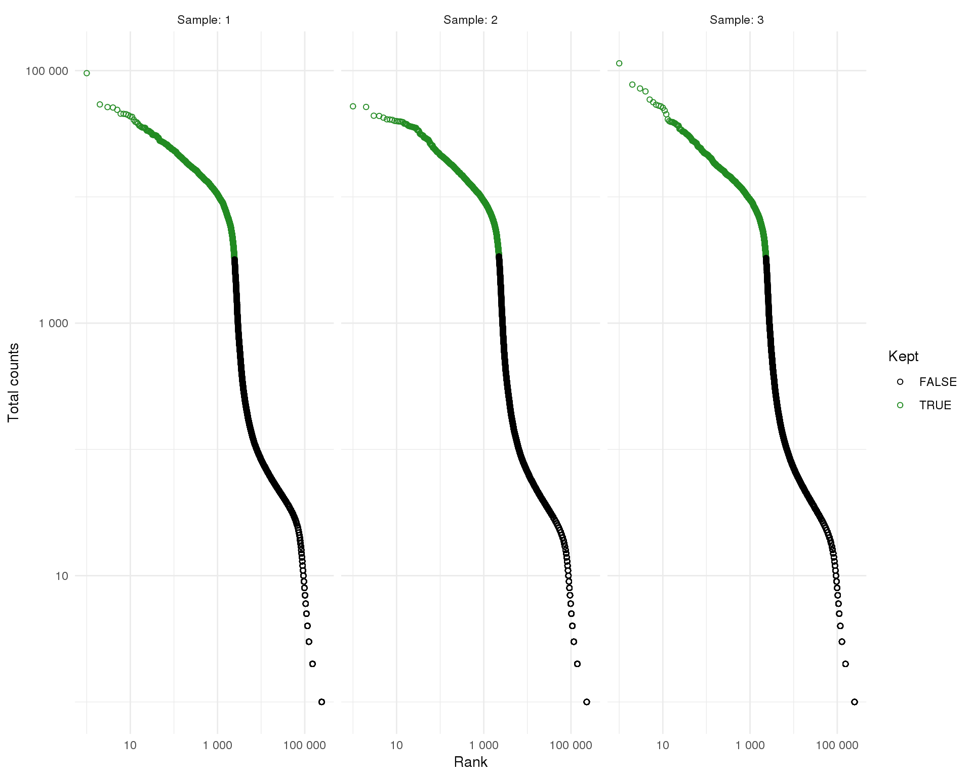
This method identifies 7006 droplets as containing cells.
Empty drops
We will now look at identifying which droplets to select using the EmptyDrops method. This method tests whether the composition of a droplet is significantly different from the ambient RNA in the sample which is obtained by pooling the empty droplets. Droplets with very large counts are also automatically retained.
set.seed(1)

emp_iters <- 30000

emp_drops <- emptyDrops(counts(raw), lower = empty_thresh, niters = emp_iters,
                        test.ambient = TRUE, BPPARAM = bpparam)
EmptyDrops calculates p-values using a permutation approach. Let’s check that we are usually a sufficient number of iterations. If there are any droplets that have non-significant p-values but are limited by the number of permuations the number should be increased.
emp_fdr <- 0.01
is_cell <- emp_drops$FDR <= emp_fdr
is_cell[is.na(is_cell)] <- FALSE

colData(raw)$EmpDropsLogProb <- emp_drops$LogProb
colData(raw)$EmpDropsPValue  <- emp_drops$PValue
colData(raw)$EmpDropsLimited <- emp_drops$Limited
colData(raw)$EmpDropsFDR     <- emp_drops$FDR
colData(raw)$EmpDropsFilt    <- is_cell

table(Limited = emp_drops$Limited, Significant = is_cell)
Significant
Limited FALSE TRUE
FALSE 935180 534
TRUE 0 9324Another way to check the EmptyDrops results is to look at the droplets below our empty threshold. We are assuming that these droplets only contain ambient RNA and therefore the null hypothesis should be true and the distribution of p-values should be approximately uniform.
colData(raw) %>%
    as.data.frame() %>%
    filter(BarcodeTotal <= empty_thresh,
           BarcodeTotal > 0) %>%
    ggplot(aes(x = EmpDropsPValue)) +
    geom_histogram() +
    xlab("p-value") +
theme_minimal()![]()
Expand here to see past versions of empty-drops-pvals-1.png:
| Version | Author | Date |
|---|---|---|
| 8f826ef | Luke Zappia | 2019-02-08 |
| 2daa7f2 | Luke Zappia | 2019-01-25 |
| b4432ff | Luke Zappia | 2019-01-18 |
Peaks near zero would tell us that not all of the droplets below the threshold are truly empty and that we should lower it.
We can also plot the negative log-probability against the total counts to see which droplets EmptyDrops has selected.
colData(raw) %>%
    as.data.frame() %>%
    filter(!is.na(EmpDropsFilt)) %>%
    ggplot(aes(x = BarcodeTotal, y = -EmpDropsLogProb, colour = EmpDropsFilt)) +
    geom_point() +
    scale_colour_discrete(name = "Significant") +
    xlab("Total counts") +
    ylab("-log(probability)") +
theme_minimal()![]()
Expand here to see past versions of empty-drops-plot-1.png:
| Version | Author | Date |
|---|---|---|
| 8f826ef | Luke Zappia | 2019-02-08 |
| 2daa7f2 | Luke Zappia | 2019-01-25 |
| b4432ff | Luke Zappia | 2019-01-18 |
| bf40049 | Luke Zappia | 2019-01-18 |
There were 923875 droplets with less than 100 counts which were used to make up the ambient RNA pool. Of the remaining 21163 droplets 9858 were found to have profiles significantly different from the ambient RNA and should contain cells.
Comparison
Let’s quickly compare differences between the selection methods using an UpSet plot:
plot_data <- list(
    "Cell Ranger"    = colData(raw)$Cell[colData(raw)$DefaultFilt],
    "Cell Ranger v3" = colData(raw)$Cell[colData(raw)$CellRangerFilt],
    "EmptyDrops"     = colData(raw)$Cell[colData(raw)$EmpDropsFilt]
)

upset(fromList(plot_data), order.by = "freq",
      sets.x.label = "Number of cells", text.scale = c(2, 1.2, 2, 1.2, 2, 3))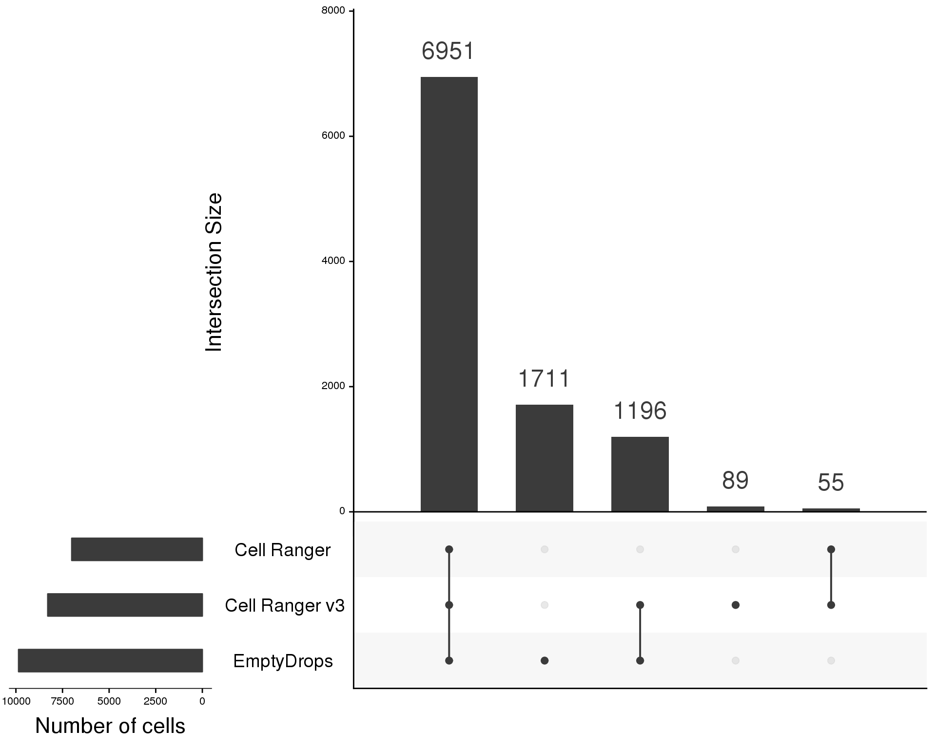
Expand here to see past versions of compare-overlap-1.png:
| Version | Author | Date |
|---|---|---|
| 4a2f376 | Luke Zappia | 2019-02-20 |
| 8f826ef | Luke Zappia | 2019-02-08 |
| 2daa7f2 | Luke Zappia | 2019-01-25 |
| b4432ff | Luke Zappia | 2019-01-18 |
| bf40049 | Luke Zappia | 2019-01-18 |
We can see that most of the cells are identified by all methods. A large number of cells are also identified by the new Cell Ranger and EmptyDrops methods. These are likely to be those cells that fall below the total counts threshold selected by the traditional Cell Ranger algorithm. Our use of the EmptyDrops algorithm has identified even more cells than Cell Ranger v3 but there are very few cells that Cell Ranger identifed which EmptyDrops didn’t.
Selection
We are going to perform further quality control of these cells anyway so at this stage we will keep those that were selected by either Cell Ranger v3 or EmptyDrops.
selected <- raw[, colData(raw)$CellRangerFilt | colData(raw)$EmpDropsFilt]
selected <- selected[Matrix::rowSums(counts(selected)) > 0, ]

colData(selected)$SelMethod <- "Both"
colData(selected)$SelMethod[!colData(selected)$CellRangerFilt] <- "emptyDrops"
colData(selected)$SelMethod[!colData(selected)$EmpDropsFilt] <- "CellRanger"
Annotation
Now that we have a dataset that just contains actual cells we will add some extra annotation. This includes downloading feature annotation from BioMart and assigning cell cycle stages using the cyclone function in the scran package as well as calculating a range of quality control metrics using scater.
selected <- annotateSCE(selected,
                        org        = "human",
                        add_anno   = TRUE,
                        host       = "jul2018.archive.ensembl.org",
                        calc_qc    = TRUE,
                        calc_cpm   = TRUE,
                        cell_cycle = TRUE,
                        BPPARAM    = bpparam)

glimpse(as.data.frame(colData(selected)))
Observations: 10,002
Variables: 55
$ Cell <chr> "Cell74", "Cell10…
$ Dataset <chr> "Orgs123", "Orgs1…
$ Barcode <chr> "AAACCTGAGAGTACAT…
$ Sample <chr> "1", "1", "1", "1…
$ CellRangerFilt <lgl> TRUE, TRUE, FALSE…
$ BarcodeRank <dbl> 2281.5, 3193.5, 1…
$ BarcodeTotal <dbl> 11084, 9414, 114,…
$ BarcodeFitted <dbl> 11089.186, 9427.9…
$ DefaultFilt <lgl> TRUE, TRUE, FALSE…
$ EmpDropsLogProb <dbl> -11721.5793, -948…
$ EmpDropsPValue <dbl> 3.333222e-05, 3.3…
$ EmpDropsLimited <lgl> TRUE, TRUE, TRUE,…
$ EmpDropsFDR <dbl> 0.000000000, 0.00…
$ EmpDropsFilt <lgl> TRUE, TRUE, TRUE,…
$ SelMethod <chr> "Both", "Both", "…
$ G1Score <dbl> 0.035, 0.398, 0.9…
$ SScore <dbl> 0.035, 0.398, 0.9…
$ G2MScore <dbl> 0.561, 0.100, 0.0…
$ CellCycle <chr> "G2M", "S", "G1",…
$ is_cell_control <lgl> FALSE, FALSE, FAL…
$ total_features_by_counts <int> 3193, 2663, 108, …
$ log10_total_features_by_counts <dbl> 3.504335, 3.42553…
$ total_counts <dbl> 11084, 9414, 114,…
$ log10_total_counts <dbl> 4.044736, 3.97382…
$ pct_counts_in_top_50_features <dbl> 31.07182, 33.8963…
$ pct_counts_in_top_100_features <dbl> 44.92061, 49.2033…
$ pct_counts_in_top_200_features <dbl> 55.37712, 59.6983…
$ pct_counts_in_top_500_features <dbl> 67.68315, 71.8398…
$ total_features_by_counts_endogenous <int> 3183, 2653, 108, …
$ log10_total_features_by_counts_endogenous <dbl> 3.502973, 3.42390…
$ total_counts_endogenous <dbl> 10647, 9142, 114,…
$ log10_total_counts_endogenous <dbl> 4.027268, 3.96108…
$ pct_counts_endogenous <dbl> 96.05738, 97.1106…
$ pct_counts_in_top_50_features_endogenous <dbl> 30.95708, 34.4891…
$ pct_counts_in_top_100_features_endogenous <dbl> 44.38809, 49.5077…
$ pct_counts_in_top_200_features_endogenous <dbl> 54.16549, 59.1227…
$ pct_counts_in_top_500_features_endogenous <dbl> 66.63849, 71.3301…
$ total_features_by_counts_feature_control <int> 10, 10, 0, 7, 10,…
$ log10_total_features_by_counts_feature_control <dbl> 1.0413927, 1.0413…
$ total_counts_feature_control <dbl> 437, 272, 0, 13, …
$ log10_total_counts_feature_control <dbl> 2.6414741, 2.4361…
$ pct_counts_feature_control <dbl> 3.9426200, 2.8893…
$ pct_counts_in_top_50_features_feature_control <dbl> 100, 100, NaN, 10…
$ pct_counts_in_top_100_features_feature_control <dbl> 100, 100, NaN, 10…
$ pct_counts_in_top_200_features_feature_control <dbl> 100, 100, NaN, 10…
$ pct_counts_in_top_500_features_feature_control <dbl> 100, 100, NaN, 10…
$ total_features_by_counts_MT <int> 10, 10, 0, 7, 10,…
$ log10_total_features_by_counts_MT <dbl> 1.0413927, 1.0413…
$ total_counts_MT <dbl> 437, 272, 0, 13, …
$ log10_total_counts_MT <dbl> 2.6414741, 2.4361…
$ pct_counts_MT <dbl> 3.9426200, 2.8893…
$ pct_counts_in_top_50_features_MT <dbl> 100, 100, NaN, 10…
$ pct_counts_in_top_100_features_MT <dbl> 100, 100, NaN, 10…
$ pct_counts_in_top_200_features_MT <dbl> 100, 100, NaN, 10…
$ pct_counts_in_top_500_features_MT <dbl> 100, 100, NaN, 10…glimpse(as.data.frame(rowData(selected)))Observations: 24,812
Variables: 20
$ ID <chr> "ENSG00000243485", "ENSG00000238009",…
$ Symbol <chr> "MIR1302-2HG", "AL627309.1", "AL62730…
$ Type <chr> "Gene Expression", "Gene Expression",…
$ Name <chr> "MIR1302-2HG", "AL627309.1", "AL62730…
$ ensembl_gene_id <chr> "ENSG00000243485", "ENSG00000238009",…
$ entrezgene <int> NA, NA, NA, NA, NA, NA, NA, NA, NA, N…
$ external_gene_name <chr> "MIR1302-2HG", "AL627309.1", "AL62730…
$ hgnc_symbol <chr> "MIR1302-2HG", "", "", "", "FAM87B", …
$ chromosome_name <chr> "1", "1", "1", "1", "1", "1", "1", "1…
$ description <chr> "MIR1302-2 host gene", "", "", "", "f…
$ gene_biotype <chr> "lincRNA", "lincRNA", "lincRNA", "lin…
$ percentage_gene_gc_content <dbl> 48.84, 39.91, 48.75, 40.42, 48.52, 52…
$ is_feature_control <lgl> FALSE, FALSE, FALSE, FALSE, FALSE, FA…
$ is_feature_control_MT <lgl> FALSE, FALSE, FALSE, FALSE, FALSE, FA…
$ mean_counts <dbl> 0.00009998, 0.00119976, 0.00019996, 0…
$ log10_mean_counts <dbl> 4.341859e-05, 5.207369e-04, 8.683285e…
$ n_cells_by_counts <int> 1, 12, 2, 379, 10, 153, 204, 12, 879,…
$ pct_dropout_by_counts <dbl> 99.99000, 99.88002, 99.98000, 96.2107…
$ total_counts <dbl> 1, 12, 2, 415, 10, 160, 214, 12, 1045…
$ log10_total_counts <dbl> 0.3010300, 1.1139434, 0.4771213, 2.61…Figure
plot_data <- colData(raw) %>%
    as.data.frame() %>%
    select(Cell, Kept = EmpDropsFilt, Rank = BarcodeRank,
           Total = BarcodeTotal, Fitted = BarcodeFitted) %>%
    arrange(Rank)

emp_plot <- plot_data %>%
    filter(Total > 0) %>%
    ggplot(aes(x = Rank, y = Total)) +
    geom_point(shape = 1, aes(colour = Kept)) +
    geom_line(aes(y = Fitted), colour = "#00B7C6", size = 1) +
    geom_hline(yintercept = bc_ranks$knee,
               colour = "#00ADEF", linetype = "dashed") +
    annotate("text", x = 0, y = bc_ranks$knee, label = "Knee",
             colour = "#00ADEF", hjust = 0, vjust = -1) +
    geom_hline(yintercept = bc_ranks$inflection,
               colour = "#8DC63F", linetype = "dashed") +
    annotate("text", x = 0, y = bc_ranks$inflection, label = "Inflection",
             colour = "#8DC63F", hjust = 0, vjust = -1) +
    geom_hline(yintercept = empty_thresh,
               colour = "#7A52C7", linetype = "dashed") +
    annotate("text", x = 0, y = empty_thresh, label = "Empty threshold",
             colour = "#7A52C7", hjust = 0, vjust = -1) +
    scale_x_log10(labels = scales::number, breaks = 10 ^ seq(0, 6)) +
    scale_y_log10(labels = scales::number, breaks = 10 ^ seq(0, 5)) +
    scale_colour_manual(values = c("black", "#EC008C"),
                        labels = c("Empty", "Cell")) +
    ggtitle("EmptyDrops droplet selection") +
    ylab("Total counts") +
    theme_minimal() +
    theme(legend.position = "bottom",
          legend.title = element_blank(),
          plot.margin = unit(c(5.5, 20, 5.5, 5.5), "points"))

ggsave(here::here("output", DOCNAME, "droplet-selection.pdf"), emp_plot,
       width = 7, height = 5, scale = 1)
ggsave(here::here("output", DOCNAME, "droplet-selection.png"), emp_plot,
       width = 7, height = 5, scale = 1)

emp_plot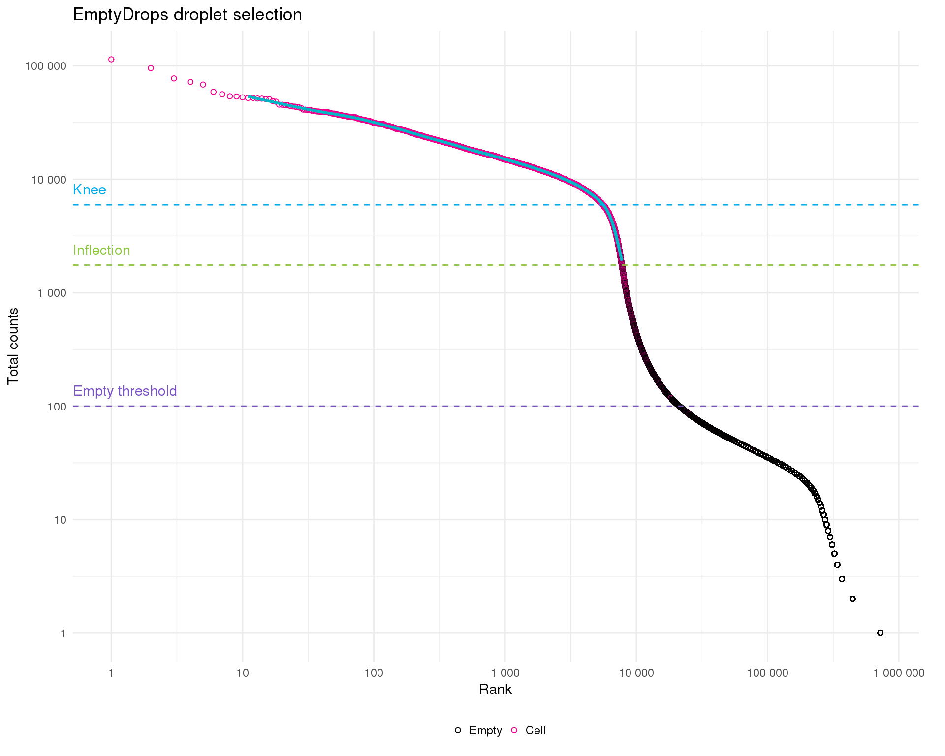
Expand here to see past versions of figure-1.png:
| Version | Author | Date |
|---|---|---|
| ae75188 | Luke Zappia | 2019-03-06 |
| 4a2f376 | Luke Zappia | 2019-02-20 |
| 431c180 | Luke Zappia | 2019-02-19 |
plot_data <- colData(raw) %>%
    as.data.frame() %>%
    select(Name             = Cell,
           `Cell Ranger`    = DefaultFilt,
           `Cell Ranger v3` = CellRangerFilt,
           EmptyDrops       = `EmpDropsFilt`,
           `Total counts`   = BarcodeTotal) %>%
    mutate(`Cell Ranger`    = if_else(`Cell Ranger`,    1L, 0L),
           `Cell Ranger v3` = if_else(`Cell Ranger v3`, 1L, 0L),
           EmptyDrops       = if_else(EmptyDrops,       1L, 0L)) %>%
    mutate(`Total counts`   = log10(`Total counts`))

upset(plot_data, order.by = "freq",
      sets.x.label = "Number of cells",
      text.scale = c(2, 1.6, 2, 1.3, 2, 3),
      matrix.color = "#7A52C7",
      main.bar.color = "#7A52C7",
      sets.bar.color = "#7A52C7")
grid.edit("arrange", name = "arrange2")
comp_plot <- grid.grab()

ggsave(here::here("output", DOCNAME, "selection-comparison.pdf"), comp_plot,
       width = 7, height = 4, scale = 1.2)
ggsave(here::here("output", DOCNAME, "selection-comparison.png"), comp_plot,
       width = 7, height = 4, scale = 1.2)
Summary
Parameters
This table describes parameters used and set in this document.
params <- list(
    list(
        Parameter = "n_droplets",
        Value = ncol(raw),
        Description = "Number of droplets in the raw dataset"
    ),
    list(
        Parameter = "empty_thresh",
        Value = empty_thresh,
        Description = "Droplets with less than this many counts are empty"
    ),
    list(
        Parameter = "emp_iters",
        Value = emp_iters,
        Description = "Number of iterations for EmptyDrops p-values"
    ),
    list(
        Parameter = "emp_fdr",
        Value = emp_fdr,
        Description = "FDR cutoff for EmptyDrops"
    ),
    list(
        Parameter = "n_default",
        Value = sum(colData(raw)$DefaultFilt),
        Description = "Number of cells selected by the default Cell Ranger method"
    ),
    list(
        Parameter = "n_cellranger",
        Value = sum(colData(raw)$CellRangerFilt),
        Description = "Number of cells selected by the Cell Ranger v3 method"
    ),
    list(
        Parameter = "n_empdrops",
        Value = sum(colData(raw)$EmpDropsFilt),
        Description = "Number of cells selected by the EmptyDrops method"
    ),
    list(
        Parameter = "n_cells",
        Value = ncol(selected),
        Description = "Number of cells selected"
    )
)

params <- jsonlite::toJSON(params, pretty = TRUE)
knitr::kable(jsonlite::fromJSON(params))| Parameter | Value | Description |
|---|---|---|
| n_droplets | 945038 | Number of droplets in the raw dataset |
| empty_thresh | 100 | Droplets with less than this many counts are empty |
| emp_iters | 30000 | Number of iterations for EmptyDrops p-values |
| emp_fdr | 0.01 | FDR cutoff for EmptyDrops |
| n_default | 7006 | Number of cells selected by the default Cell Ranger method |
| n_cellranger | 8291 | Number of cells selected by the Cell Ranger v3 method |
| n_empdrops | 9858 | Number of cells selected by the EmptyDrops method |
| n_cells | 10002 | Number of cells selected |
Output files
This table describes the output files produced by this document. Right click and Save Link As… to download the results.
write_rds(selected, here::here("data/processed/01-selected.Rds"))dir.create(here::here("output", DOCNAME), showWarnings = FALSE)
for (sample in unique(colData(selected)$Sample)) {
barcodes <- colData(selected) %>%
as.data.frame() %>%
filter(Sample == sample) %>%
select(Barcode) %>%
mutate(Barcode = paste0(Barcode, "-1"))
readr::write_tsv(barcodes,
print(here::here("output", DOCNAME,
glue::glue("barcodes_Org{sample}.tsv"))),
col_names = FALSE)
}readr::write_lines(params, here::here("output", DOCNAME, "parameters.json"))
knitr::kable(data.frame(
File = c(
getDownloadLink("parameters.json", DOCNAME),
getDownloadLink("barcodes_Org1.tsv", DOCNAME),
getDownloadLink("barcodes_Org2.tsv", DOCNAME),
getDownloadLink("barcodes_Org3.tsv", DOCNAME),
getDownloadLink("droplet-selection.png", DOCNAME),
getDownloadLink("droplet-selection.pdf", DOCNAME),
getDownloadLink("selection-comparison.png", DOCNAME),
getDownloadLink("selection-comparison.pdf", DOCNAME)
),
Description = c(
"Parameters set and used in this analysis",
"Selected barcodes for organoid 1",
"Selected barcodes for organoid 2",
"Selected barcodes for organoid 3",
"Droplet selection figure (PNG)",
"Droplet selection figure (PDF)",
"Selection comparison figure (PNG)",
"Selection comparison figure (PDF)"
)
))| File | Description |
|---|---|
| parameters.json | Parameters set and used in this analysis |
| barcodes_Org1.tsv | Selected barcodes for organoid 1 |
| barcodes_Org2.tsv | Selected barcodes for organoid 2 |
| barcodes_Org3.tsv | Selected barcodes for organoid 3 |
| droplet-selection.png | Droplet selection figure (PNG) |
| droplet-selection.pdf | Droplet selection figure (PDF) |
| selection-comparison.png | Selection comparison figure (PNG) |
| selection-comparison.pdf | Selection comparison figure (PDF) |
Session information
devtools::session_info()─ Session info ──────────────────────────────────────────────────────────
setting value
version R version 3.5.0 (2018-04-23)
os CentOS release 6.7 (Final)
system x86_64, linux-gnu
ui X11
language (EN)
collate en_US.UTF-8
ctype en_US.UTF-8
tz Australia/Melbourne
date 2019-04-03
─ Packages ──────────────────────────────────────────────────────────────
! package * version date lib source
assertthat 0.2.0 2017-04-11 [1] CRAN (R 3.5.0)
backports 1.1.3 2018-12-14 [1] CRAN (R 3.5.0)
bindr 0.1.1 2018-03-13 [1] CRAN (R 3.5.0)
bindrcpp 0.2.2 2018-03-29 [1] CRAN (R 3.5.0)
Biobase * 2.42.0 2018-10-30 [1] Bioconductor
BiocGenerics * 0.28.0 2018-10-30 [1] Bioconductor
BiocParallel * 1.16.5 2019-01-04 [1] Bioconductor
bitops 1.0-6 2013-08-17 [1] CRAN (R 3.5.0)
broom 0.5.1 2018-12-05 [1] CRAN (R 3.5.0)
callr 3.1.1 2018-12-21 [1] CRAN (R 3.5.0)
cellranger 1.1.0 2016-07-27 [1] CRAN (R 3.5.0)
cli 1.0.1 2018-09-25 [1] CRAN (R 3.5.0)
colorspace 1.4-0 2019-01-13 [1] CRAN (R 3.5.0)
cowplot * 0.9.4 2019-01-08 [1] CRAN (R 3.5.0)
crayon 1.3.4 2017-09-16 [1] CRAN (R 3.5.0)
DelayedArray * 0.8.0 2018-10-30 [1] Bioconductor
desc 1.2.0 2018-05-01 [1] CRAN (R 3.5.0)
devtools 2.0.1 2018-10-26 [1] CRAN (R 3.5.0)
digest 0.6.18 2018-10-10 [1] CRAN (R 3.5.0)
dplyr * 0.7.8 2018-11-10 [1] CRAN (R 3.5.0)
DropletUtils * 1.2.2 2019-01-04 [1] Bioconductor
edgeR 3.24.3 2019-01-02 [1] Bioconductor
evaluate 0.12 2018-10-09 [1] CRAN (R 3.5.0)
forcats * 0.3.0 2018-02-19 [1] CRAN (R 3.5.0)
fs 1.2.6 2018-08-23 [1] CRAN (R 3.5.0)
generics 0.0.2 2018-11-29 [1] CRAN (R 3.5.0)
GenomeInfoDb * 1.18.1 2018-11-12 [1] Bioconductor
GenomeInfoDbData 1.2.0 2019-01-15 [1] Bioconductor
GenomicRanges * 1.34.0 2018-10-30 [1] Bioconductor
ggplot2 * 3.1.0 2018-10-25 [1] CRAN (R 3.5.0)
git2r 0.24.0 2019-01-07 [1] CRAN (R 3.5.0)
glue 1.3.0 2018-07-17 [1] CRAN (R 3.5.0)
gridExtra 2.3 2017-09-09 [1] CRAN (R 3.5.0)
gtable 0.2.0 2016-02-26 [1] CRAN (R 3.5.0)
haven 2.0.0 2018-11-22 [1] CRAN (R 3.5.0)
HDF5Array 1.10.1 2018-12-05 [1] Bioconductor
here 0.1 2017-05-28 [1] CRAN (R 3.5.0)
hms 0.4.2 2018-03-10 [1] CRAN (R 3.5.0)
htmltools 0.3.6 2017-04-28 [1] CRAN (R 3.5.0)
httr 1.4.0 2018-12-11 [1] CRAN (R 3.5.0)
IRanges * 2.16.0 2018-10-30 [1] Bioconductor
jsonlite 1.6 2018-12-07 [1] CRAN (R 3.5.0)
knitr 1.21 2018-12-10 [1] CRAN (R 3.5.0)
P lattice 0.20-35 2017-03-25 [5] CRAN (R 3.5.0)
lazyeval 0.2.1 2017-10-29 [1] CRAN (R 3.5.0)
limma 3.38.3 2018-12-02 [1] Bioconductor
locfit 1.5-9.1 2013-04-20 [1] CRAN (R 3.5.0)
lubridate 1.7.4 2018-04-11 [1] CRAN (R 3.5.0)
magrittr 1.5 2014-11-22 [1] CRAN (R 3.5.0)
P Matrix 1.2-14 2018-04-09 [5] CRAN (R 3.5.0)
matrixStats * 0.54.0 2018-07-23 [1] CRAN (R 3.5.0)
memoise 1.1.0 2017-04-21 [1] CRAN (R 3.5.0)
modelr 0.1.3 2019-02-05 [1] CRAN (R 3.5.0)
munsell 0.5.0 2018-06-12 [1] CRAN (R 3.5.0)
P nlme 3.1-137 2018-04-07 [5] CRAN (R 3.5.0)
pillar 1.3.1 2018-12-15 [1] CRAN (R 3.5.0)
pkgbuild 1.0.2 2018-10-16 [1] CRAN (R 3.5.0)
pkgconfig 2.0.2 2018-08-16 [1] CRAN (R 3.5.0)
pkgload 1.0.2 2018-10-29 [1] CRAN (R 3.5.0)
plyr 1.8.4 2016-06-08 [1] CRAN (R 3.5.0)
prettyunits 1.0.2 2015-07-13 [1] CRAN (R 3.5.0)
processx 3.2.1 2018-12-05 [1] CRAN (R 3.5.0)
ps 1.3.0 2018-12-21 [1] CRAN (R 3.5.0)
purrr * 0.3.0 2019-01-27 [1] CRAN (R 3.5.0)
R.methodsS3 1.7.1 2016-02-16 [1] CRAN (R 3.5.0)
R.oo 1.22.0 2018-04-22 [1] CRAN (R 3.5.0)
R.utils 2.7.0 2018-08-27 [1] CRAN (R 3.5.0)
R6 2.3.0 2018-10-04 [1] CRAN (R 3.5.0)
Rcpp 1.0.0 2018-11-07 [1] CRAN (R 3.5.0)
RCurl 1.95-4.11 2018-07-15 [1] CRAN (R 3.5.0)
readr * 1.3.1 2018-12-21 [1] CRAN (R 3.5.0)
readxl 1.2.0 2018-12-19 [1] CRAN (R 3.5.0)
remotes 2.0.2 2018-10-30 [1] CRAN (R 3.5.0)
rhdf5 2.26.2 2019-01-02 [1] Bioconductor
Rhdf5lib 1.4.2 2018-12-03 [1] Bioconductor
rlang 0.3.1 2019-01-08 [1] CRAN (R 3.5.0)
rmarkdown 1.11 2018-12-08 [1] CRAN (R 3.5.0)
rprojroot 1.3-2 2018-01-03 [1] CRAN (R 3.5.0)
rstudioapi 0.9.0 2019-01-09 [1] CRAN (R 3.5.0)
rvest 0.3.2 2016-06-17 [1] CRAN (R 3.5.0)
S4Vectors * 0.20.1 2018-11-09 [1] Bioconductor
scales 1.0.0 2018-08-09 [1] CRAN (R 3.5.0)
sessioninfo 1.1.1 2018-11-05 [1] CRAN (R 3.5.0)
SingleCellExperiment * 1.4.1 2019-01-04 [1] Bioconductor
stringi 1.2.4 2018-07-20 [1] CRAN (R 3.5.0)
stringr * 1.3.1 2018-05-10 [1] CRAN (R 3.5.0)
SummarizedExperiment * 1.12.0 2018-10-30 [1] Bioconductor
testthat 2.0.1 2018-10-13 [4] CRAN (R 3.5.0)
tibble * 2.0.1 2019-01-12 [1] CRAN (R 3.5.0)
tidyr * 0.8.2 2018-10-28 [1] CRAN (R 3.5.0)
tidyselect 0.2.5 2018-10-11 [1] CRAN (R 3.5.0)
tidyverse * 1.2.1 2017-11-14 [1] CRAN (R 3.5.0)
UpSetR * 1.3.3 2017-03-21 [1] CRAN (R 3.5.0)
usethis 1.4.0 2018-08-14 [1] CRAN (R 3.5.0)
whisker 0.3-2 2013-04-28 [1] CRAN (R 3.5.0)
withr 2.1.2 2018-03-15 [1] CRAN (R 3.5.0)
workflowr 1.1.1 2018-07-06 [1] CRAN (R 3.5.0)
xfun 0.4 2018-10-23 [1] CRAN (R 3.5.0)
xml2 1.2.0 2018-01-24 [1] CRAN (R 3.5.0)
XVector 0.22.0 2018-10-30 [1] Bioconductor
yaml 2.2.0 2018-07-25 [1] CRAN (R 3.5.0)
zlibbioc 1.28.0 2018-10-30 [1] Bioconductor
[1] /group/bioi1/luke/analysis/phd-thesis-analysis/packrat/lib/x86_64-pc-linux-gnu/3.5.0
[2] /group/bioi1/luke/analysis/phd-thesis-analysis/packrat/lib-ext/x86_64-pc-linux-gnu/3.5.0
[3] /group/bioi1/luke/analysis/phd-thesis-analysis/packrat/lib-R/x86_64-pc-linux-gnu/3.5.0
[4] /home/luke.zappia/R/x86_64-pc-linux-gnu-library/3.5
[5] /usr/local/installed/R/3.5.0/lib64/R/library
P ── Loaded and on-disk path mismatch.This reproducible R Markdown analysis was created with workflowr 1.1.1