Chapter 1 Introduction

See, people they don’t understand

No, girlfriends, they can’t understand

Your grandsons, they won’t understand

On top of this, I ain’t ever gonna understand…

— The Strokes

Last Nite, 2001

This introduction chapter provides the background and overview necessary for understanding my work in this thesis, including an introduction to basic cell biology and kidney development, the technologies we use to measure those processes in the cell and the computational methods we use to analyse the data these technologies produce. Section 1.1 - The central dogma describes how information flows within a cell and the molecules involved in these processes. Section 1.2 - RNA sequencing covers the technologies used to measure the dynamic changes in some of these molecules and the established computational methods that are commonly used to extract meaning from this kind of data. In Section 1.3 - Single-cell RNA sequencing I discuss new technologies that have enabled measurements on the level of individual cells while Section 1.4 - Analysing scRNA-seq data outlines the types of analysis that can be performed on this data and the tools and methods that perform them. Section 1.5 - Kidney development provides a brief introduction to kidney structure and development and how it can be studied using stem cell technologies. This section provides background for Chapter 5 where I describe an analysis of a dataset from developing kidney organoids. My introduction ends with Section 1.6 - Thesis overview and aims which presents an overview of my thesis aims and how I have completed them in the following chapters. An online version of this thesis is available at https://lazappi.github.io/phd-thesis/.

1.1 The central dogma

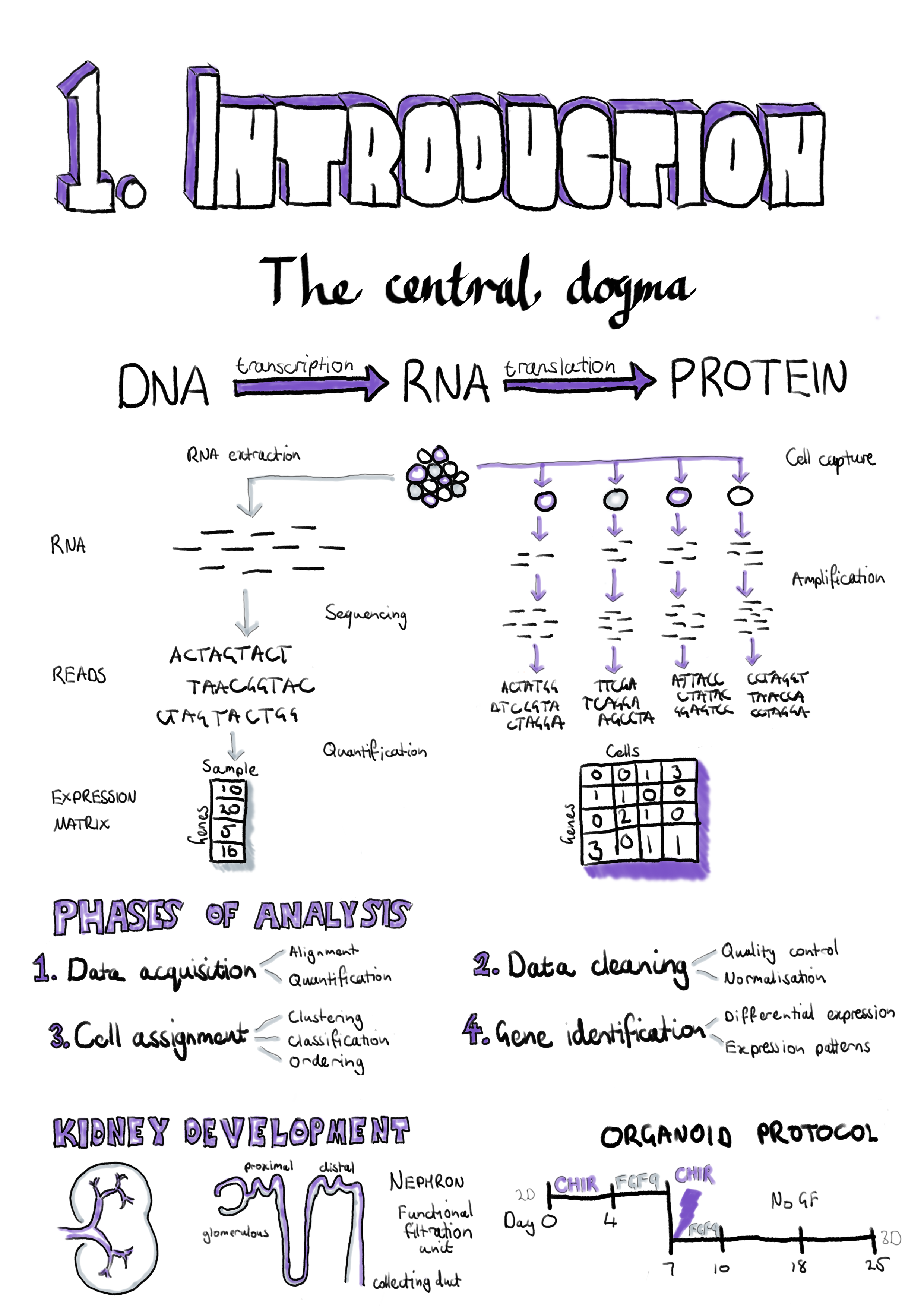
The central dogma of molecular biology describes the flow of information within a cell, from DNA to RNA to protein (Figure 1.1). Deoxyribonucleic acid (DNA) is the long-term data storage of the cell and has a well-known double helix structure [1–3]. Each strand of the double helix consists of a series of nucleotide molecules linked by phosphate groups. These nucleotides are made of three subunits: a nitrogenous base, a deoxyribose sugar and a phosphate group. DNA nucleotides come in four species, adenine, cytosine, thymine and guanine, which have different base subunits. The sugar and phosphate groups form the backbone of each DNA strand and the two strands are bound together through hydrogen bonds between matching nucleotides known as base pairs. Guanine forms three hydrogen bonds with cytosine and adenine forms two with thymine. In computing terms DNA is similar to a hard drive in that it provides stable, consistent storage of important information.

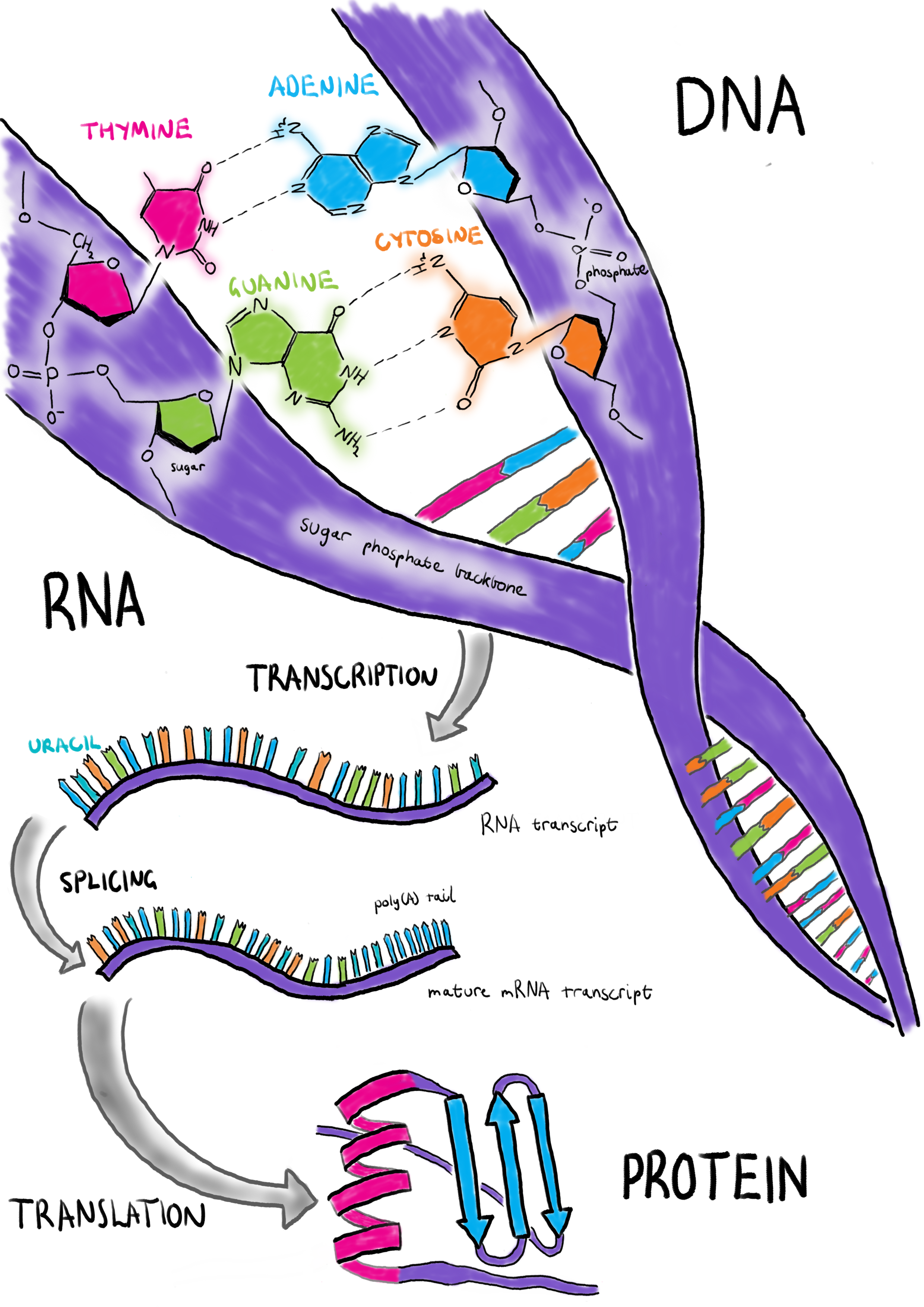
Figure 1.1: The central dogma of molecular biology. Deoxyribonucleic acid (DNA) is the long-term data storage of the cell. To use this information a ribonucleic acid (RNA) molecule is produced through a process called transcription. A mature messenger RNA (mRNA) requires splicing and addition of a ploy(A) tail. Proteins are created from mRNA through translation in the ribosome.

When the cell wants to use some of this information it produces a copy of it in the form of a ribonucleic acid (RNA) molecule through a process known as transcription, similar to a computer loading information it wants to use into its random access memory. Sections of DNA that encode functional information are called genes. RNA is similar to a single strand of DNA except that the deoxyribose sugar is replaced with ribose and the thymine nucleotide is replaced with another nucleotide called uracil. Because it is single-stranded, RNA does not have a double helix structure but it can form complex shapes by binding to itself. A cell is able to create many copies of the same RNA molecule and this is referred to as the expression level. By varying RNA expression the activity of processes within a cell can be regulated. There are several different types of RNA that serve different purposes. RNA molecules that are transcribed from protein-coding genes are known as messenger RNA (mRNA). Other types of RNA include ribosomal RNA (rRNA) which forms part of the ribosome (the molecular machinery that manufactures proteins), transfer RNA (tRNA) which carries amino acids to the ribosome, micro RNA (miRNA) which have a role in regulating gene expression and long non-coding RNA (lncRNA) which are also involved in regulation among other processes. Genes are made up of regions that encode information (known as exons) that alternate with much larger non-coding regions (introns).

When an mRNA molecule is transcribed it initially contains the intronic sequences but these are removed through a process known as RNA splicing and a sequence of adenine nucleotides (a poly(A) tail) is added where transcription ends (the 3’ end) to mark a mature mRNA molecule. This splicing process allows multiple forms of a protein to be produced from a single gene by selecting which exons are retained or removed. A mature mRNA transcript is converted to a protein in a complex structure called the ribosome which is made up of specialised RNA and proteins. The conversion process is known as translation because the information encoded by nucleic acids in RNA is translated to information stored as amino acids in the protein. Proteins complete most of the work required to keep a cell functioning and can be compared to the programs running on a computer. These functions require complex three dimensional structures and include tasks such as sensing things in the external environment, transporting nutrients into the cell, regulating the expression of genes, constructing new proteins, recycling molecules and facilitating metabolism. Understanding the molecules involved in the central dogma is central to our understanding of how a cell works.

1.2 RNA sequencing

By looking at DNA we can see what versions of genes are present in a cell but we cannot tell which of them are active and what processes they might be involved in. To do that we need to inspect the parts of the system that change dynamically. Ideally we might want to interrogate the proteins that are present, as they provide most of the functionality. However, while it is possible to do this using technologies such as mass spectrometry the readout produced is more difficult to interpret and the encoding is much more complex as there are 20 different amino acids compared to only four nucleotides. In contrast, RNA molecules are much easier to measure. High-throughput RNA sequencing (RNA-seq) provides a reliable method for high-quality measurement of RNA expression levels. RNA is isolated from a biological sample, converted to complementary DNA (cDNA) and provided as input to a sequencing machine. The output of an RNA-seq experiment is millions of short nucleotide sequences originating from the RNA transcripts present in the sample. Compared to older techniques for measuring RNA, such as probe-based microarrays, RNA-seq requires no prior knowledge of existing sequences in order to measure a sample and is effective over a much greater range of expression levels.

1.2.1 Library preparation

The first step in preparing a sample for RNA-seq is to chemically lyse the cells, disrupting the structure of the cell wall and releasing the molecules inside. RNA molecules can then be isolated, typically using a chemical process called phenol/chloroform extraction, although this can also be done by physically separating different types of molecules by passing the sample through a silica column. The majority of the RNA in a cell is ribosomal RNA, usually more than 80 percent [4]. Most of the time this type of RNA is not of interest and because the total amount of sequencing in an experiment is limited sequencing rRNA would reduce the ability to detect less abundant species. To select mature mRNA transcripts, oligonucleotide probes that bind to the poly(A) tail can be used, but a downside of this approach is that it won’t capture immature mRNA or other types of RNA molecules. An alternative method is ribosomal RNA depletion where a different kind of probe specific to each species is used that binds to the rRNA allowing it to be removed. The choice of selection method has been shown to introduce different biases into the resulting data [5].

The Illumina sequencing typically used for RNA-seq experiments can only read short sequences of nucleotides of approximately 40–400 base pairs. Most mRNA molecules are longer than this so to read the full length of a transcript it must first be fragmented into smaller parts. Most sequencing machines also only work with DNA, not directly with RNA, so the sample must first be reverse-transcribed using a retroviral enzyme to produce a single strand of cDNA. Many protocols have been designed for this step with each requiring a specific primer sequence to be joined to the RNA molecules. The complementary strand of cDNA is produced using a second enzyme that is usually involved in copying DNA for cell division. For some protocols fragmentation is performed after conversion to cDNA rather than at the RNA stage.

Once the cDNA has been produced it is usually necessary to attach adaptor sequences that are used to bind the molecules and initiate sequencing (Figure 1.2). These adaptors may also contain multiplexing barcodes that tag all the molecules in a sample and allow multiple samples to be sequenced at once. It has become standard practice to perform paired-end sequencing, where a section of nucleotides is read from one end of a fragment before it is flipped and the other end read, and this process requires an additional set of adaptors. At each of the stages of library preparation there are quality control steps to be performed to make sure a high-quality cDNA sample is loaded on to the sequencing machine.

Figure 1.2: Illustration of adapter arrangements for the Illumina platform ((A) minimal adapter components, (B) “in-line” barcode configuration for paired-end sequencing, (C) index configuration for paired-end sequencing). Sequencing primers SP1 (primary) and SP2 (paired-end) allow initiation of synthesis of the insert sequence. Index or barcode sequences allow multiplexing of multiple samples with the index being sequenced from a separate index primer (IP). (Image adapted from RNA-seqlopedia, http://rnaseq.uoregon.edu [6]).

1.2.2 High-throughput sequencing

Most RNA-seq experiments are sequenced on an Illumina machine using their Sequence by Synthesis technology (Figure 1.3). In this process the two strands of cDNA fragments are separated and the adaptors bind to oligonucleotides probes coating a flow cell. The other end of the fragment can bind to a second oligonucleotide forming a bridge structure where an enzyme synthesises the complementary DNA strand. This process of separation of strands and synthesis of new complementary strands is repeated until clusters of DNA fragments with the same sequence are formed. Once the clusters contain enough fragments the adaptor at one end of each fragment is cleaved leaving single-stranded DNA attached to the flow cell at one end.

Figure 1.3: The Illumina Sequencing by Synthesis process. Nucleotide fragments bind to a flow cell and clusters are formed through bridge amplification. Strands are primed and nucleotides tagged with fluorescent labels are added to the flow cell along with a DNA polymerase enzyme. The lanes of the flow cell are then scanned to produce an image. The fluorescent tags are cleaved and 3’-OH blocking groups are added, preparing the strands for another round of nucleotide incorporation. Image adapted from Mardis, “Next-Generation DNA Sequencing Methods” [7].

The sequencing process now begins. Nucleotides tagged with fluorescent markers are added and can bind to the next available position on a fragment if they are complementary. By adding all four nucleotides at once they compete for each position, reducing the chance of an incorrect match. Any unbound nucleotides are washed away before a laser excites the fluorescent tags and an image is taken. Each nucleotide is tagged with a different colour and the order of colours produced by a cluster shows the sequence of nucleotides in a fragment. For paired-end sequencing the fragments can be flipped and the sequencing process repeated at the other end. The images from the sequencing machine are processed to produce millions of short nucleotide sequences known as reads that are the starting point for computational analysis.

1.2.3 Analysis of RNA-seq data

Many types of analyses can be performed using RNA-seq data, such as identification of variants in the genetic sequence or detection of previously unannotated transcripts, but the most common kind of analysis is to look for differences in the expression level of genes between groups of samples (Figure 1.4). To do this, reads are first aligned to a reference genome and the number of reads overlapping each gene is counted. In contrast to aligners designed for DNA sequencing, RNA-seq aligners such as STAR [8], HISAT2 [9] and subread [10] must take into account the splicing structure of mRNA transcripts which causes parts of some reads to align in different locations in the genome. The alignment step is computationally intensive and can take a significant amount of time. More recently tools such as kallisto [11] and Salmon [12] have been developed which attempt to directly quantify expression by estimating the probability that a read comes from a particular annotated transcript. These approaches are orders of magnitude faster than true genome alignment and potentially produce more accurate quantification, at the cost of having an exact genomic position for each read.

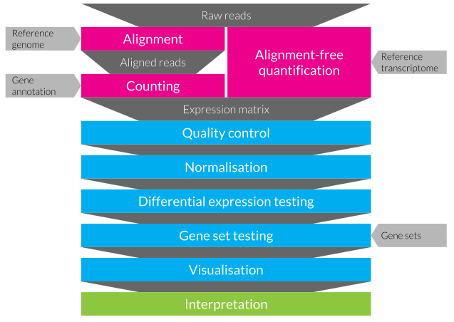
Figure 1.4: A typical RNA-seq differential expression testing workflow. An expression matrix is created from raw reads either by aligning them to a reference genome and counting those that overlap annotated genes or by alignment-free quantification (pink). Data analysis (blue) consists of several steps including quality control of samples and features, normalisation to remove technical differences between samples, testing for differential expression, gene set testing to identify enriched signatures, and visualisation. Results must be carefully interpreted (green) to extract meaning.

At this stage the result is a matrix of counts, known as an expression matrix, where the rows are features (usually genes), the columns are samples and the values show the expression level of a particular feature in a sample. As these counts result from a sampling process they can be modelled using common statistical distributions. One option is the Poisson distribution which describes the probability of a given number of events happening in a fixed amount of time, however this distribution assumes that the mean and variance of each feature is equal. This can be true for replicates of the same RNA-seq sample but does not represent the extra biological variability between different samples [13]. A better fit is the negative binomial (or Gamma-Poisson) distribution which includes an over-dispersion parameter, allowing the variance in expression to be larger than the mean. While each feature is quantified for each sample, the observed expression levels are related to the total number of reads and the expression level of other features. For example, if a gene is highly expressed in a particular sample it will soak up a large proportion of the available reads, while in another sample where it is less expressed those reads are more likely to be sampled from other genes. Another complication of RNA-seq data is that the number of features (tens of thousands) is much larger than the number of samples (usually only a few per group) which violates the assumptions of many traditional statistical techniques. Technical variation is another well-known problem in high-throughput genomics studies, for example it has been estimated that only 17.8 percent of allele-specific expression is due to biological variation with the rest being technical noise [14].

Both the edgeR [15,16] and DESeq [17] (and later the DESeq2 [18]) packages model RNA-seq data using the negative binomial distribution, but before differences in expression levels are tested the technical differences between samples should be removed through normalisation. Early approaches include simple transformations like Reads (or Fragments) Per Kilobase per Million (RPKM/FPKM) [19] or Transcripts Per Million (TPM) [20] which correct for the total number of reads per cell and gene length. The edgeR package uses the Trimmed-Mean of M values (TMM) method where a scaling factor for each sample is produced using the weighted mean of log ratios between samples for each gene, after excluding the highest expressed genes and those with the largest log ratio [13]. DESeq has a similar method that uses the median of the ratio of the expression of each gene to the geometric mean expression across all samples. The limma package [21] uses an alternative approach where a method called voom transforms the data so that it is suitable for linear modelling methods originally designed for RNA microarray technology [22]. When an experiment has been conducted in multiple batches and there are significant differences between them, alternative normalisation methods such as Remove Unwanted Variation (RUV) may be required [23]. RUV estimates unknown factors of unwanted variation using negative control genes (genes that are expected to be consistent between samples). These factors can then be included in the generalised linear modelling frameworks used for testing differential expression. Over time the methods in these packages have been refined and new tests developed allowing for the routine analysis of many RNA-seq experiments.

1.3 Single-cell RNA sequencing

Traditional bulk RNA-seq experiments average the transcriptome across the millions of cells in a sample. Recently it has become possible to perform single-cell RNA sequencing (scRNA-seq) and investigate the transcriptome at the resolution of individual cells. There are many situations where it is important to understand how specific cell types react to development or perturbations. This is often hindered in bulk analyses which may be affected by the unknown proportions of cell types in a sample. Studies into gene expression in specific cell types previously required selecting and isolating the cells of interest, which separates them from the other cell types they are usually associated with and makes it impossible to investigate interactions between them. With scRNA-seq technologies it is now possible to look at the transcriptome of all the cell types in a tissue simultaneously, which has led to a better understanding of what makes cell types distinct and the discovery of previously unknown cell types.

1.3.1 Early single-cell capture technologies

The first scRNA-seq protocol was published in 2009 [24], just a year after the first bulk RNA-seq publication [19]. While this approach allowed measurements of the transcriptome in individual cells it required manual manipulation and was restricted to inspecting a few precious cells. Further studies quickly showed that cell types could be identified without sorting cells and approaches were developed to allow unbiased capture of the whole transcriptome. Since then, many scRNA-seq protocols have been developed (including CEL-Seq [25], CEL-Seq2 [26], Quartz-Seq [27], Quartz-Seq2 [28] and Smart-seq2 [29]) and the number of cells in scRNA-seq experiments has scaled exponentially (Figure 1.5) [30]. The first commercially available cell capture platform was the Fluidigm C1. This system uses microfluidics to passively separate cells into individual wells on a plate where they are lysed, reverse transcribed and the collected cDNA is PCR amplified. After this stage the product is extracted from the plate and libraries prepared for Illumina sequencing. Most C1 data has been produced using a 96 well plate but more recently an 800 well plate has become available, greatly increasing the number of cells that can be captured at a time. One of the disadvantages of microfluidic plate-based cell capture technologies is that the chips used have a fixed size window, meaning that only cells of a particular sizes can be captured in a single run. However, as cells are captured in individual wells they can be imaged before lysis, potentially identifying damaged or broken cells, empty wells or wells containing more than one cell. Capturing multiple cells is a known issue, with Macosko et al. finding that when preparing a mixture of mouse and human cells, 30 percent of the resulting libraries contained transcripts from both species but only about a third of these doublets were visible in microscopy images [31]. The newer Polaris system from Fluidigm also uses microfluidics to capture cells but can select particular cells based on staining or fluorescent reporter expression and then hold them for up to 24 hours while introducing various stimuli. The cells can be imaged during this time before being lysed and prepared for RNA sequencing. This platform provides opportunities for a range of experiments that aren’t possible using other capture technologies.

Figure 1.5: Exponential increase in the scale of scRNA-seq experiments. (a) Key jumps in scRNA-seq capture technologies including manual handling, plate-based microfluidic capture and droplet-based capture. (b) Cell numbers in representative studies using key technologies by publication date. Image from Svensson, Vento-Tormo and Teichmann “Exponential scaling of single-cell RNA-seq in the past decade” [30].

1.3.2 Droplet-based cell capture

An alternative to using microfluidics to capture cells in wells is to capture them in nano-droplets. In this process a dissociated cell mixture is fed into a microfluidic device, while beads coated in primers enter at another input. The device is designed to form aqueous droplets within mineral oil and the inputs are arranged so that cells and beads can be simultaneously captured within a droplet. When this happens the reagents carried along with the bead lyse the cell and any poly(A) tagged RNA molecules present can bind to the capture probes on the bead. Reverse transcription and PCR amplification then begins and an individual cDNA library is produced for each cell, tagged with the unique barcode sequence present on the bead. The main advantage of droplet-based capture technologies is the ability to capture many more cells at one time, up to tens of thousands. These approaches are also less selective about cell size and produce fewer doublets. As a result they are much cheaper per cell, although as sequencing costs are fixed studies using droplet-based captures typically sequence individual cells at a much lower depth.

Droplet-based capture was popularised by the publication of the Drop-seq [31] and InDrop [32] platforms in 2015 and the updated InDrops in 2017 [33]. These are both DIY systems and although they differ in how the beads are produced, when the droplets are broken and in some aspects of the chemistry they can both be constructed on a lab bench from syringes, automatic plungers, a microscope and a small custom-made microfluidic chip. A similar commercially available platform is the 10x Genomics Chromium device which automates and streamlines much of the process (Figure 1.6) [34]. This device uses droplet-based technologies for a range of applications including capture of cells for scRNA-seq. More specialised captures, such as those aimed at profiling immune cell receptors, are also possible and the company has recently announced kits for single-cell Assay for Transposase-Accessible Chromatin using sequencing (scATAC-seq) capture. A recent review has suggested that the 10x Chromium provides the most appropriate droplet-based capture for most experiments that aren’t cost sensitive or require custom protocols [35].

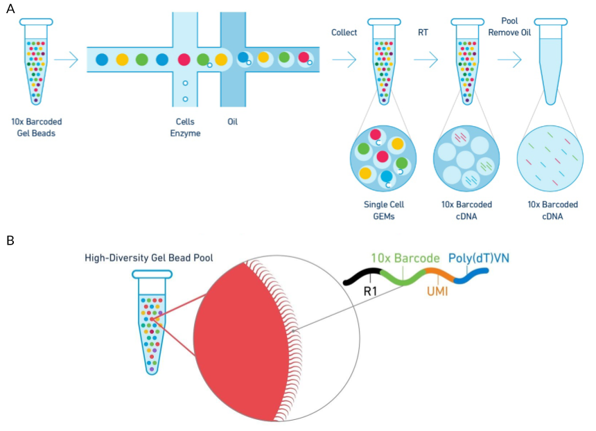
Figure 1.6: Diagram of the 10x Genomics Chromium cell capture process. (A) Steps in the cell capture process. Barcoded gel beads are passed into a microfluidic device along with dissociated cells where they are captured in aqueous droplets in an oil solution. Cells are lysed within the droplets and mRNA is reverse transcribed to produced barcoded cDNA. Droplets are then broken and the cDNA collected for sequencing. (B) Structure of the gel bead capture probe including adaptor, cell barcode, UMI and poly(T) tail. Adapted using images from 10x Genomics.

1.3.3 Unique Molecular Identifiers

In contrast to plate-based capture methods, which usually provide reads along the length of RNA transcripts, droplet-based capture methods typically employ protocols which include short random nucleotide sequences known as Unique Molecular Identifiers (UMIs) [36]. Individual cells contain very small amounts of RNA (around 10–30 pg, less than 5 percent of which is mRNA) and to obtain enough cDNA for sequencing a PCR amplification step is necessary. Depending on their nucleotide sequence different transcripts may be amplified at different rates which can distort their relative proportions within a library. UMIs attempt to improve the quantification of gene expression by allowing the removal of PCR duplicates produced during amplification (Figure 1.7) [37]. The nucleotide probes used in droplet-based capture protocols include a poly(T) sequence which binds to mature mRNA molecules, a barcode sequence which is the same for every probe on a bead and 8–10 bases of UMI sequence which is unique to each probe. The UMI sequences are long enough that the probability of capturing two copies of a transcript on two probes with the same UMI is extremely low. After reverse transcription, amplification, sequencing and alignment, de-duplication can be performed by identifying reads with the same UMI that align to the same position and therefore should be PCR duplicates rather than truly expressed copies of a transcript.

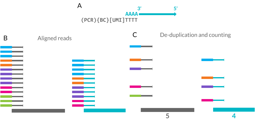
Figure 1.7: Unique Molecular Identifiers (UMIs) can improve scRNA-seq quantification. (A) UMIs are random 8–10 base pair sequences included as part of the mRNA capture probe along with the cell barcode (BC) and PCR handle. (B) The mRNA sequence can be aligned to a reference genome. (C) Each UMI is only counted once at each location, removing PCR duplicates and improving quantification.

For this method to be effective each read must be associated with a UMI which means that only a small section at the 3’ end of each transcript is sequenced. This has the side effect of reducing the amount of cDNA that needs to be sequenced and therefore increasing the number of cells that can be sequenced at a time. While the improvement in quantification of gene expression levels is useful for many downstream analyses, it comes at the cost of coverage across the length of a transcript, which is required for applications such as variant detection and de-novo assembly. However, reads along the length of genes have been observed in UMI datasets and are believed to come from unannotated transcription start sites or regions that contain enough adenine nucleotides to bind to the capture probes. Datasets with UMIs need extra processing steps which can be complicated by the possibility of sequencing errors in the UMI itself. Statistical methods designed for full-length data may also be affected by the different properties of a UMI dataset.

1.3.4 Recent advances in scRNA-seq protocols

Although droplet-based techniques are currently the most commonly used cell capture technologies, other approaches have been proposed that promise to capture even more cells at a lower cost per cell. These include approaches based around sub-nanolitre sized wells, for example the Seq-Well protocol [38]. A simple flow cell is constructed with an array of microwells made from polydimethylsiloxane (PDMS), a silicone rubber. A solution containing dissociated cells is flowed over the array and cells are captured in the wells by gravity. This is repeated to capture barcoded beads before adding reagents and sealing the wells. Once reactions are complete the beads can be retrieved and processed in a similar way to droplet-based capture [39]. Some cell types are difficult to capture due to their size, shape or other properties, and in some cases, particularly in tissues such as the brain, it has been suggested that single-nucleus rather than single-cell RNA-seq may be more effective [40–43]. In these protocols Nuclei are captured and processed in a similar way to cells, however the RNA within them is immature and unspliced so different reference annotations are required during analysis.

Extensions to the standard protocols have also been proposed that allow multiple measurements from the same cell (Figure 1.8). One such protocol is CITE-seq which enables measurement of the levels of selected proteins at the same time as the whole transcriptome (Figure 1.9A) [44]. Antibodies for the proteins of interest are labelled with short nucleotide sequences. These antibodies can then be applied to the dissociated cells and any that remain unbound are washed away before cell capture. The antibody labels are then captured along with mRNA transcripts and a size selection step is applied to separate them before library preparation. Similar antibodies can be used to allow multiplexing of samples through a process known as cell hashing (Figure 1.9B) [45]. In a typical scRNA-seq experiment each batch corresponds to a single sample. This complicates analysis as it is impossible to tell what is noise due to cells being processed in the same way and what is true biological signal. Cell hashing uses an antibody to a ubiquitously expressed protein but with a different nucleotide sequence for each sample. The samples can then be mixed, processed in batches and then the cells computationally separated based on which sequence they are associated with. An added benefit of this approach is the simple detection of doublets containing cells from different samples.

Figure 1.8: The range of multimodal scRNA-seq technologies. Many protocols have been developed to enable multiple measurements from the same individual cells with a selection shown here. These other measurements (shaded colours) include genotype (rose bud), methylation (cornsilk), chromatin state (muted lime), transcription factor binding (periwinkle), protein expression (jade lime), activation or repression (cabbage), lineage tracing (aquamarine blue), spatial location (light sky blue) or electrophysiology (cotton candy). Image from https://github.com/arnavm/multimodal-scRNA-seq available under a Creative Commons Attribution-NonCommercial-ShareAlike 4.0 International (CC BY-NC-SA 4.0) license [46].

Figure 1.9: Extensions to droplet-based capture protocols using nucleotide tagged antibodies. (A) CITE-seq allows measurement of selected cell surface markers along with the transcriptome. Nucleotide tagged antibodies are applied to cells before droplet-based capture and processing. A size selection step is used to separate antibody nucleotides before library preparation. (B) Cell hashing allows multiplexing of samples. Ubiquitous antibodies are used to tag cells in each sample with a hashtag oligonucleotide. The cells are then mixed for cell capture and processing and the hashtags used to computationally identify the origin of each cell. Images from https://cite-seq.com [47].

CRISPR-Cas9 gene editing has also been developed as an extension to scRNA-seq protocols. One possibility is to introduce a mutation at a known location that can then be used to demultiplex samples processed together [48]. It is possible to do this with samples from different individuals or cell lines but the advantage of a gene editing based approach is that the genetic background remains similar between samples. It is also possible to investigate the effects of introducing a mutation. Protocols like Perturb-Seq [49] introduce a range of guide RNA molecules to a cell culture, subject the cells to some stimulus then perform single-cell RNA sequencing. The introduced mutation can then be linked to the response of the cells to the stimulus and the associated broader changes in gene expression. More recently it has been proposed that CITE-seq can be combined with CRISPR-based approaches [50]. Another approach is CellTagging which introduces a barcoded lentiviral construct into cells [51]. A unique combination of barcodes is then passed on to daughter cells and can be used to trace the lineage of a cell population.

Other approaches that allow multiple measurements from the same individual cells include G&T-seq [52] and SIDR [53] which measure RNA and genomic DNA, similar approaches which measure the exome (or protein-coding part of the genome) along with the transcriptome [54], scMT-seq which measures RNA and DNA methylation [55], Patch-seq which combines patch-clamp recording to measure the electrophysiology of neurons with scRNA-seq [56] and scTrio-seq which is able to measure the genome, transcriptome and methylome simultaneously [57].

1.4 Analysing scRNA-seq data

Cell capture technologies and scRNA-seq protocols have developed rapidly but the data they produce still presents a number of challenges. Existing approaches are inefficient, capturing around 10 percent of transcripts in a cell [58]. When combined with the low sequencing depth per cell this results in a limited sensitivity and an inability to detect lowly expressed transcripts. The small amount of starting material also contributes to high levels of technical noise, complicating downstream analysis and making it difficult to detect biological differences [59]. In order to capture cells they must first be dissociated into single-cell suspensions but this step can be non-trivial. Some tissues or cell types may be more difficult to separate than others and the treatments required to break them apart may affect the health of the cells and their transcriptional profiles. It has been suggested that damage caused by dissociation can be minimised by using a cold-active protease to separate cells [60]. Other cell types may be too big or have other characteristics that prevent them being captured. Multiple cells may be captured together or empty wells or droplets sequenced making quality control of datasets an important consideration.

As well as increasing technical noise the small amounts of starting material and low sequencing depth mean there are many occasions where zero counts are recorded, indicating no measured expression for a particular gene in a particular cell. These zero counts often represent the true biological state we are interested in as we that different genes will be expressed by different cell types. However, zeros can also be the result of confounding biological factors such as stage in the cell cycle, transcriptional bursting and environmental interactions which cause genuine changes in expression but that might not be of interest to a particular study. On top of this there are effects that are purely technical factors. In particular, sampling effects, which can result in “dropout” events where a transcript is truly expressed in a sample but is not observed in the sequencing data [61]. In bulk experiments these effects are limited by averaging across the cells in a sample and by the greater sequencing depth, but for single-cell experiments they can present a significant challenge for analysis as methods must account for the missing information and the large number of zeros may cause the assumptions of existing methods to be violated.

One approach to tackling the problem of too many zeros is to use zero-inflated versions of common distributions [62–65]. However, it is still debatable whether scRNA-seq datasets, particularly those from droplet-based capture protocols [66], are truly zero inflated or if the additional zeros are better modelled with standard distributions with lower means. Another approach to analysis is to impute some of the zeros, replacing them with estimates of how expressed those genes truly are based on their expression in similar cells using methods such as MAGIC [67], SAVER [68,69] or scImpute [70]. However, imputation comes with the risk of introducing false structure that is not actually present in the samples [71].

Bulk RNA-seq experiments usually involve predefined groups of samples, for example cancer cells and normal tissue, different tissue types or treatment and control groups. It is possible to design scRNA-seq experiments in the same way by sorting cells into known groups based on surface markers, sampling them at a series of time points or comparing treatment groups, but often single-cell experiments are more exploratory. Many of the single-cell studies to date have sampled developing or mature tissues and attempted to profile the cell types that are present [32,72–77]. This approach is best exemplified by the Human Cell Atlas project which is attempting to produce a reference of the transcriptional profiles of all the cell types in the human body [78]. Similar projects exist for other species and specific tissues [79–88].

As scRNA-seq datasets have become more widely available, a standard analysis workflow has developed which can be applied to many experiments [89,90]. This workflow can be divided into four phases shown in Figure 1.10: 1) Data acquisition, pre-processing of samples to produce a cell by gene expression matrix, 2) Data cleaning, quality control to refine the dataset used for analysis, 3) Cell assignment, grouping or ordering of cells based on their transcriptional profile, and 4) Gene identification to find genes that represent particular groups and can be used to interpret them. Within each phase a range of processes may be used and there are now many tools available for completing each of them, with over 450 tools currently available. An introduction to the phases of scRNA-seq analysis is provided here but the analysis tools landscape is more fully explored in Chapter 2.

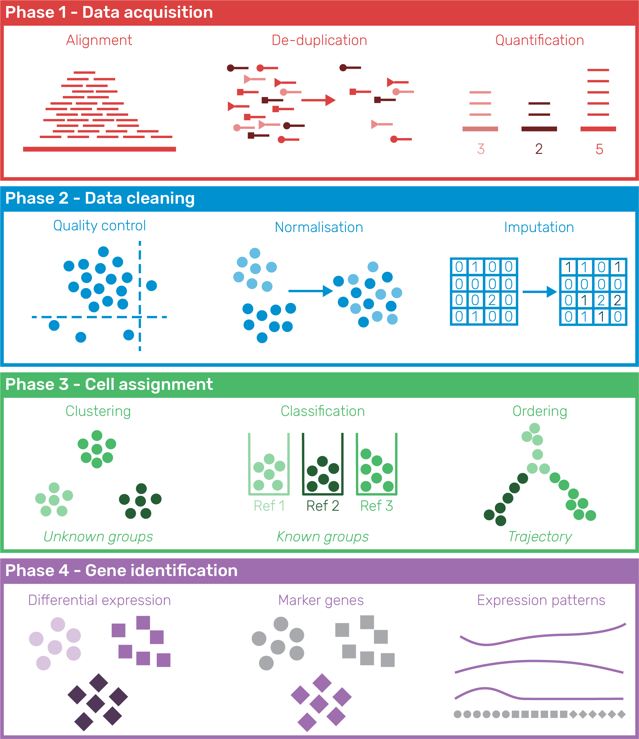
Figure 1.10: Phases of a standard scRNA-seq analysis workflow. In Phase 1 (Data acquisition) samples are pre-processed to produce an expression matrix that undergoes quality control and filtering in Phase 2 (Data cleaning). Phase 3 (Cell assignment) groups or orders cells according to their transcriptional profile and in Phase 4 (Gene identification) genes describing those groups are discovered and used to interpret them.

1.4.1 Pre-processing and quality control

The result of a sequencing experiment is typically a set of image files from the sequencer or a FASTQ file containing nucleotide reads but for most analyses we use an expression matrix where each column is a cell, each row is a feature and the values indicate expression levels. To produce this matrix there is a series of pre-processing steps, typically beginning will some quality control of the raw reads. Reads are then aligned to a reference genome and the number of reads overlapping annotated features (genes or transcripts) is counted. Probabilistic quantification methods can be applied to full-length scRNA-seq datasets but have required adaptations such as the alevin method for UMI-based datasets [91] in the Salmon package. When using conventional alignment, UMI samples need extra processing with tools like UMI-tools [92], umis [93] or zUMIs [94] in order to assign cell barcodes and deduplicate UMIs. For datasets produced using the 10x Chromium platform the company provides the Cell Ranger software which is a complete pre-processing pipeline that also includes an automated downstream analysis. Other packages such as scPipe [95] also aim to streamline this process with some such as Falco [96] designed to work on scalable cloud-based infrastructure which may be required as bigger datasets continue to be produced.

Quality control of individual cells is important as experiments will contain low-quality cells that can be uninformative or lead to misleading results. Particular types of cells that are commonly removed include damaged cells, doublets where multiple cells have been captured together [97,98] and empty droplets or wells that have been sequenced but do not contain a cell [99]. Quality control can be performed on various levels including the quality scores of the reads themselves and how or where they align to features of the expression matrix. The Cellity package attempts to automate this process by inspecting a series of biological and technical features and using machine learning methods to distinguish between high and low-quality cells [100]. However, the authors found that many of the features were cell type specific and more work needs to be done to make this approach more generally applicable. The scater package [101] emphasises a more exploratory approach to quality control at the expression matrix level by providing a series of functions for visualising various features of a dataset. These plots can then be used for selecting thresholds for removing cells. Plate-based capture platforms can produce additional biases based on the location of individual wells, a problem which is addressed by the OEFinder package which attempts to identify and visualise these “ordering effects”[102].

Filtering and selection of features also deserves attention. Genes or transcripts that are lowly expressed are typically removed from datasets in order to reduce computational time and the effect of multiple-testing correction but it is unclear how many counts indicate that a gene is truly “expressed”. Many downstream analyses operate on a selected subset of genes and how they are selected can have a dramatic effect on their results [103]. These features are often selected based on how variable they are across the dataset but this may be a result of noise rather than biological importance. Alternative selection methods have been proposed such as M3Drop which identifies genes that have more zeros than would be expected based on their mean expression [104].

1.4.2 Normalisation and integration

Effective normalisation is just as crucial for single-cell experiments as it is for bulk RNA-seq datasets. FPKM or TPM transformations can be used, but for UMI data the gene length correction is not required as reads only come from the ends of transcripts [105]. Normalisation methods designed for detecting differential expression between bulk samples such as TMM or the DESeq method can be applied, but it is unclear how suitable they in the single-cell context. Many of the early normalisation methods developed specifically for scRNA-seq data made use of spike-ins. These are synthetic RNA sequences added to cells in known quantities such as the External RNA Controls Consortium (ERCC) control mixes, a set of 92 transcripts from 250 to 2000 base pairs long based on bacterial plasmids. Brennecke et al. [106], Ding et al. [107] and Grün, Kester and van Oudenaarden [58] all propose methods for estimating technical variance using spike-ins, as does Bayesian Analysis of Single-Cell Sequencing data (BASiCS) [108]. Using spike-ins for normalisation assumes that they properly capture the dynamics of the underlying dataset and even if this is the case it is restricted to protocols where they can be added which does not include droplet-based capture techniques. The scran package implements a method that doesn’t rely on spike-ins, instead using a pooling approach to compensate for the large number of zero counts where expression levels are summed across similar cells before calculating size factors that are deconvolved back to the original cells [109]. The BASiCS method has also been adapted to experiments without spike-ins by integrating data replicated across batches [110], but only for designed experiments where groups are known in advance.

Early scRNA-seq studies often made use of only a single sample but as technologies have become cheaper and more widely available it is common to see studies with multiple batches or making use of publicly available data produced by other groups. While this expands the potential insights to be gained it presents a problem as to how to integrate these datasets [111]. A range of computational approaches for performing integration have been developed including bbknn [112], ClusterMap [113], kBET [114], LIGER [115], matchSCore [116], Scanorama [117] and scMerge [118]. The alignment approach in the Seurat package [119] uses Canonical Correlation Analysis (CCA) [120] to identify a multi-dimensional subspace that is consistent between datasets. Dynamic Time Warping (DTW) [122] is then used to stretch and align these dimensions so that the datasets are similarly spread along them. Some tasks can be performed using these aligned dimensions, but as the original expression matrix is unchanged the integration is not used for other tasks such as differential expression testing. The authors of scran use a Mutual Nearest Neighbours (MNN) approach that calculates a cosine distance between cells in different datasets then identifies those that share a neighbourhood [123]. Batch correction vectors can then be calculated and subtracted from one dataset to overlay them. A recent update to the Seurat method combines these approaches by applying CCA before using the MNN approach to identify “anchor” cells that have common features in the different datasets [124].

1.4.3 Grouping cells

Grouping similar cells is a key step in analysing scRNA-seq datasets that is not usually required for bulk experiments and as such it has been a key focus of methods development. Over one hundred tools have been released for clustering cells which attempt to address a range of technical and biological challenges [125]. Some of these methods include SINgle CEll RNA-seq profiling Analysis (SINCERA) [126], Single-Cell Consensus Clustering (SC3) [127], single-cell latent variable model (scLVM) [76] and Spanning-tree Progression Analysis of Density-normalised Events (SPADE) [128], as well as BackSPIN which was used to identify nine cell types and 47 distinct subclasses in the mouse cortex and hippocampus in one of the earliest studies to demonstrate the possibilities of scRNA-seq [72]. All of these tools attempt to cluster similar cells together based on their expression profiles, forming groups of cells of the same type. The clustering method in the Seurat package [129] has become particularly popular and has been shown to perform well, particularly on UMI datasets [130,131]. This method begins by selecting a set of highly variable genes then performing PCA on them. A set of dimensions is then selected that contains most of the variation in the dataset. Alternatively, if Seurat’s alignment method has been used to integrate datasets the aligned CCA dimensions are used instead. Next, a Shared Nearest Neighbours (SNN) graph is constructed by considering the distance between cells in this multidimensional space and the overlap between shared neighbourhoods. Seurat uses a Euclidean distance but it has been suggested that correlations can provide better results [132]. In order to separate cells into clusters, a community detection algorithm such as Louvain optimisation [133] is run on the graph with a resolution parameter that controls the number of clusters that are produced. Selecting this parameter and similar parameters in other methods is difficult but important as the number of clusters selected can affect the interpretation of results. I address this problem with a visualisation-based approach in Chapter 4.

For tissue types that are well understood or where comprehensive references are available an alternative to unsupervised clustering is to directly classify cells. This can be done using a gating approach based on the expression of known marker genes similar to that commonly used for flow cytometry experiments. Alternatively, machine learning algorithms can be used to perform classification based on the overall expression profile. Methods such as scmap [134], scPred [135], CaSTLe [136] and Moana [137] take this approach. Classification has the advantage of making use of existing knowledge and avoids manual annotation and interpretation of clusters which can often be difficult and time consuming. However, it is biased by what is present in the reference datasets used and typically cannot reveal previously unknown cell types or states. As projects like the Human Cell Atlas produce well-annotated references based on scRNA-seq data the viability of classification and other reference-based methods will improve.

1.4.4 Ordering cells

In some studies, for example in development where stem cells are differentiating into mature cell types, it may make sense to order cells along a continuous trajectory from one cell type to another instead of assigning them to distinct groups. Trajectory analysis was pioneered by the Monocle package which used dimensionality reduction and computation of a minimum spanning tree to explore a model of skeletal muscle differentiation [77]. Since then the Monocle algorithm has been updated [138] and a range of others developed including TSCAN [139], SLICER [140], CellTree [141], Sincell [142], Mpath [143] and Slingshot [144]. In their review of trajectory inference methods, Cannoodt, Saelens and Saeys break the process into two steps (Figure 1.11) [145]. In the first step, dimensionality reduction techniques such as principal component analysis (PCA) [146], t-distributed stochastic neighbourhood embedding (t-SNE) [147] or uniform manifold approximation and projection (UMAP) [148] are used to project cells into lower dimensions where the cells are clustered or a graph constructed between them. The trajectory is then created by finding a path through the cells and ordering the cells along it. The same group of authors have conducted a comprehensive comparison of ordering methods evaluating their performance on a range of real and synthetic datasets [149]. To do so the authors had to develop metrics for comparing trajectories from different methods and built a comprehensive infrastructure for running and evaluating software tools. They found that the performance of methods depended on the underlying topology of the data and that multiple complementary trajectory inference approaches should be used to better what is occurring.

Figure 1.11: Trajectory inference framework as described by Cannoodt, Saelens and Saeys. In the first stage, dimensionality reduction is used to convert the data to a simpler representation. In the second stage a trajectory is identified and the cells ordered. Image from Cannoodt, Saelens and Saeys “Computational methods for trajectory inference from single-cell transcriptomics” [145].

An alternative continuous approach is the cell velocity technique [150] introduced for scRNA-seq data in the velocyto package [151]. RNA-seq studies typically focus on the expression of mature mRNA molecules but a sample will also contain immature mRNA that are yet to be spliced. Examining the reads assigned to introns can indicate newly transcribed mRNA molecules and therefore which genes are currently active. Instead of assigning cells to discrete groups or along a continuous path velocyto uses reads from unspliced regions to place them in a space and create a vector indicating the direction in which the transcriptional profile is heading. This vector can show that a cell is differentiating in a particular way or that a specific transcriptional program has been activated.

Deciding on which cell assignment approach to use depends on the source of the data, the goals of the study and the questions that are being asked. Both grouping and ordering can be informative and it is often useful to attempt both on a dataset and see how they compare.

1.4.5 Gene detection and interpretation

Once cells are assigned by clustering or ordering the problem is to interpret what these groups represent. For clustered datasets this is usually done by identifying genes that are differentially expressed across the groups or marker genes that are expressed in a single cluster. Many methods have been suggested for testing differential expression, some of which take in to account the unique features of scRNA-seq data, for example D3E [152], DEsingle [65], MAST [153], scDD [154] and SCDE [155]. The large number of cells in scRNA-seq datasets means that some of the problems that made standard statistical tests unsuitable for bulk RNA-seq experiments do not apply. Simple methods like the unpaired Wilcoxon rank-sum test (or Mann-Whitney U test), Student’s t-test or logistic regression may give reasonable results in this setting. Methods originally developed for bulk experiments have also been applied to scRNA-seq datasets but the assumptions they make may not be appropriate for single-cell data. Methods such as ZINB-WaVe [64] may be required to transform the data so that bulk testing methods are appropriate. A comprehensive evaluation of 36 differential expression testing approaches found that methods developed for bulk RNA-seq did not perform worse than scRNA-seq specific methods, however, the performance of bulk methods depended on how lowly-expressed genes were filtered [156]. The authors also observed that some methods were biased in the types of features they tended to detect as differentially expressed. Often the goal is not to find all the genes that are differentially expressed between groups but to identify genes which uniquely mark particular clusters. This goal is open to alternative approaches, such as the Gini coefficient which measures unequal distribution across a population. Another approach is to construct machine learning classifiers for each gene to distinguish between one group and all other cells. Genes that give good classification performance should be good indicators of what is specific to that cluster. It is also possible to identify genes that might have the same mean between groups but differ in variance or other characteristics of their expression distribution.

When cells have been ordered along a continuous trajectory the task is slightly different. Instead of testing for a difference in means between two groups, the goal is to find genes that have a relationship between expression and pseudotime. This can be accomplished by fitting splines to the relationship between pseudotime and expression and testing the fitting coefficients. For more complex trajectories it can also be useful to find genes that are differently expressed along each side of a branch point. Monocle’s BEAM (Branch Expression Analysis Modelling) method does this using a likelihood ratio test between splines where the branch assignments are known or unknown [157]. Genes that are associated with a trajectory are important in their own right as they describe the biology along a path but they can also be used to identify cell types at end points.

Interpreting the meaning of detected marker genes is a difficult task and is likely to remain so. Some methods have been developed for this task such as celaref which suggests cluster labels based on similarity of marker genes to an already characterised reference dataset. Gene set testing to identify related categories such as Gene Ontology terms can also help but often it is necessary to rely on the results of previous functional studies. Ultimately this can only be reliably done by working closely with experts who have significant domain knowledge in the cell types being studied. An additional concern for unsupervised scRNA-seq studies is that the same genes are used for clustering or ordering and determining what those clusters or trajectories mean. This is a problem addressed by Zhang, Kamath and Tse who suggest a differential expression test using a long-tailed distribution for testing genes following clustering [158].

1.4.6 Alternative analyses

Some uses of scRNA-seq data fall outside the most common workflow and methods have been developed for a range of other purposes. For example, methods have been designed for assigning haplotypes to cells [159], detecting allele-specific expression [160–162], identifying alternative splicing [163–165] or calling single nucleotide or complex genomic variants [166–168]. Other methods have been designed for specific cell types or tissues such as reconstructing immune cell receptors on B-cells (BraCeR [169], BRAPeS [170], VDJPuzzle [171]) or T-cells (TraCeR [172], TRAPeS [173]) or interrogating the development of cancer samples (HoneyBADGER [174], SSrGE [166]). Most future studies can be expected to continue to follow common practice but it is also expected that researchers will continue to push the boundaries of what it is possible to study using scRNA-seq technologies.

1.4.7 Evaluation of scRNA-seq analysis methods

Although the analysis for many scRNA-seq studies follow a standard workflow there is wide variation in the tools that are used. We are now at the stage where there are multiple software packages for completing every stage of analysis. Deciding which tools to use can be difficult and depends on a number of factors including effectiveness, robustness, scalability, availability, ease of use and quality of documentation. In terms of effectiveness, publications describing analysis methods should demonstrate two things: 1) they can perform the task they are designed for (at least as well as existing methods) and 2) performing that task leads to biological insights. Answering the first question is difficult using real datasets as often the underlying truth is not known. For this reason simulation techniques are commonly used to produce synthetic datasets in order to evaluate methods. I present a software package for simulating scRNA-seq data in Chapter 3. Simulation is an efficient and flexible approach for producing gold standard datasets but synthetic data can never fully reproduce a real dataset. An alternative approach is to carefully construct a gold standard biological dataset by combining samples where the true differences are known [175]. These datasets can be extremely useful but are difficult, time-consuming and expensive to produce and can only reproduce a limited set of scenarios. Comprehensive evaluations of methods have already been conducted for some aspects of scRNA-seq analysis including clustering [130,131], trajectory inference [149] and differential expression testing [156] but these will need to continue to be performed and updated as the field matures and new methods are developed.

1.5 Kidney development

One area that has particularly benefitted from the possibilities created by scRNA-seq technology is developmental biology. Although the genes involved in the development of many organs are now well understood, arriving at this knowledge has required many painstaking experiments to investigate a single gene at a time. During development cells are participating in a continuous dynamic process involving the maturation from one cell type to another and the creation of new cell types. Single-cell RNA-seq captures a snapshot of the expression of all the genes involved in this process, allowing the transcriptome of intermediate and mature cells to be studied. This has revealed that some of the genes thought to be markers of specific cell types are more widely expressed or involved in other processes.

1.5.1 Structure and function

The kidney is the organ responsible for filtering the blood in order to remove waste products. In humans, kidneys grow as a pair of functional organs with each being around the size of an adult fist and weighing about 150 grams. Blood flows into the kidney via the renal artery and the blood vessels form a tree-like branching structure with ever smaller capillaries (Figure 1.12A). At the end of these branches are nephrons, the functional filtration unit of the kidney (Figure 1.12B). Humans can have around 1 million nephrons [176] that are formed during development and just after birth, however they cannot be regenerated during adulthood. A capillary loop is formed inside a structure at the end of the nephron called a glomerulus and surrounded by Bowman’s capsule. Here specialised cells called podocytes create a structure called the slit diaphragm that allows water, metal ions and small molecules to be filtered while keeping blood cells and larger species such as proteins trapped within the bloodstream. The rest of the nephron is divided into segments that are responsible for different processes involved in balancing the concentration of these species in the filtrate (Figure 1.12C). The tubular segments of the nephron are surrounded by capillaries, allowing molecules to be transferred between the filtrate and blood as required. The first segment of the nephron is the proximal tubule. Here common biomolecules such as glucose, amino acids and bicarbonate are reabsorbed into the bloodstream, as is most of the water present. Other molecules including urea and ammonium ions are secreted from the blood into the filtrate at his stage. The proximal tubule is followed by the loop of Henle and the distal tubule where ions are reabsorbed including potassium, chlorine, magnesium and calcium. The final segment is the collecting duct where salt concentrations are balanced by exchanging sodium in the filtrate for potassium in the bloodstream using a process controlled by the hormone aldosterone. The remaining filtrate is then passed to the ureter where it is carried to the bladder and collected as urine while the blood leaves via the renal vein. In order to perform this complex series of reabsorption and secretion steps, each segment of the nephron is made up specialised cell types with their own sets of signalling and transporter proteins. The filtration process is repeated about 12 times every hour with around 200 litres of blood being filtered during a day. Aside from removing waste and maintaining the balance of molecular species in the bloodstream, the kidneys also play a role in the activation of vitamin D. Other important functions include synthesising the hormones erythropoietin, which stimulates red blood cell production, and renin, which is part of the pathway that controls fluid volume and the constriction of arteries to regulate blood pressure.

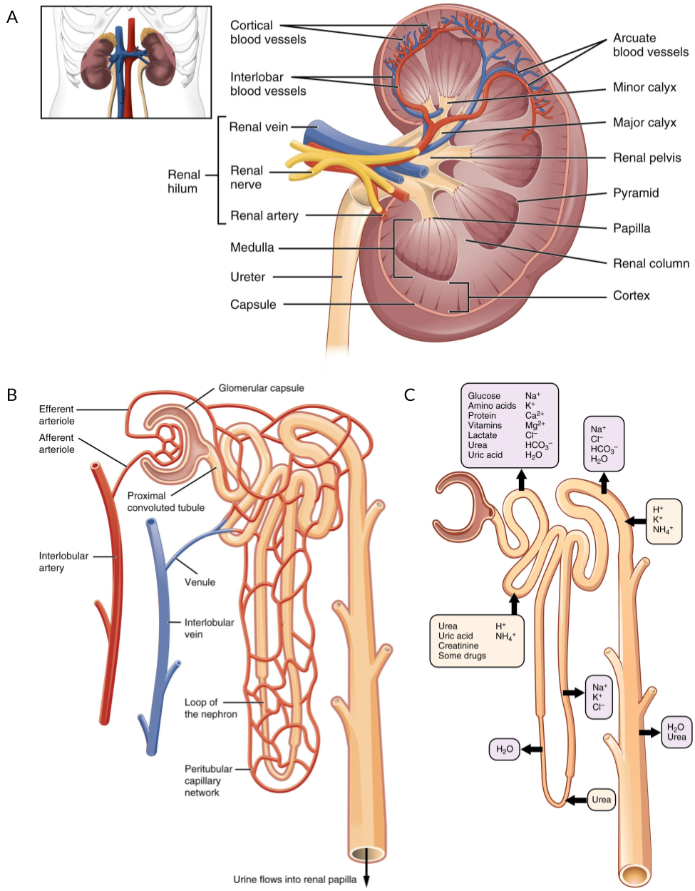
Figure 1.12: Structure of the kidney and nephron. (A) Blood flows into the kidney via the renal artery which branches into ever smaller capillaries. (B) At the end of these capillaries is the nephron, the functional filtration unit of the kidney, which is surrounded by a capillary network. (C) Different segments of the kidney are responsible for transferring specific molecular species between the bloodstream and the filtrate. Figure adapted using images from OpenStax College via Wikimedia Commons under a CC BY 3.0 license.

Chronic kidney disease is a major health problem in Australia with 1 percent of the population (237800 people) diagnosed with it in 2017 [177] and it being considered a contributory factor for 13 percent of deaths [178]. Early stages of the disease can be managed but once it becomes severe the only treatment options are dialysis, which is expensive, time consuming and unpleasant, or a kidney transplant. There are also a range of genetic developmental kidney disorders that have limited treatment options and can profoundly affect quality of life. Understanding how the kidney grows and develops is key to developing new treatments that may improve kidney function or repair damage.

1.5.2 Stages of development

The kidney develops from a region of the early embryo called the intermediate mesoderm and occurs in three phases with a specific spatial and temporal order [179]. The first phase results in the pronephros which consists of 6–10 pairs of tubules that forms the mature kidney in most primitive vertebrates such as hagfish. By about the fourth week of human embryonic development this structure dies off and is replaced by the mesonephros, which is the form of kidney present in most fish and amphibians. The mesonephros is functional during weeks 4–8 of human embryonic development before degenerating, although parts of its duct system go on to form part of the male reproductive system. The final phase of human kidney development results in the metanephros which begins developing at around five weeks and continues to around week 36 to become the permanent and functional kidney [180]. Individual nephrons grow in a similar series of stages. Cells from the duct that will become the ureter begin to invade the surrounding metanephric mesenchyme forming a ureteric bud. Interactions between these cell types, including Wnt signalling, cause mesenchymal cells to condense around the ureteric bud forming a stem cell population known as the cap mesenchyme, which expresses genes such as Six2 and Cited1. Cells from the cap mesenchyme first form a renal vesicle, a primitive structure with a lumen, which extends to form an S-shaped body (Figure 1.13). By this stage the lumen has joined with the ureteric bud to form a continuous tubule. The s-shaped body continues to elongate with podocytes beginning to develop and form a glomerulus at one end and other specialised cells arising along the length of the tubule to form the various nephron segments. Several signalling pathways and cell–cell interactions are involved in this process, including Notch signalling. While all nephrons form before birth they continue to elongate and mature postnatally.

Figure 1.13: Diagram of the stages of nephron maturation. The nephron begins as a pre-tubular aggregate (PA) which forms a renal vesicle (RV), comma-shaped body (CSB), S-shaped body (SSB), capillary loop nephron and mature nephron. The connection between the forming nephron and the lumen of the adjacent ureteric epithelium forms at late renal vesicle stage. Adapted from Little “Improving our resolution of kidney morphogenesis across time and space” [180].

Most of our understanding of kidney development comes from studies using mouse models and other model species. While these have greatly added to our knowledge they do not completely replicate human kidney development and there are known to be significant differences in the developmental timeline, signalling pathways and gene expression between species [181]. To better understand human kidney development we need models that reproduce the human version of this process.

1.5.3 Growing kidney organoids

One alternative model of human kidney development is to grow miniature organs in a lab. Known as organoids, these tissues are grown from pluripotent stem cells provided with the right sequence of conditions and growth factors [182]. Naturally occurring embryonic stem cells can be used but a more feasible approach is to reprogram mature cell types (typically fibroblasts from skin samples) using a method discovered by Takahashi and Yamanaka [183,184]. Under this protocol, cells are supplied with the transcription factors Oct3/4, Sox2 and Klf4 using retroviral transduction. The resulting cells have the ability to differentiate into any cell type and are known as induced pluripotent stem cells (iPSCs). By culturing iPSCs under the right conditions the course of differentiation can be directed, and protocols for growing a range of tissues have been developed including stomach, intestine, liver, lung and brain [185]. The first protocol for growing kidney organoids was published in 2015 by Takasato et al. (Figure 1.14) [186].

Figure 1.14: Diagram of the Takasato et al. kidney organoid protocol. iPSCs are cultured on a plate in the presence of CHIR followed by FGF9. After about a week cells are formed into three-dimensional pellets and a short CHIR pulse is applied. The pellets continue to be cultured in FGF9 for a further 10 days before all growth factors are removed. The organoids now contain tubular structures replicating human nephrons. Adapted from Takasato et al. “Kidney organoids from human iPS cells contain multiple lineages and model human nephrogenesis” [186].

Using this protocol, iPSCs are first grown on a plate where Wnt signalling is induced by the presence of CHIR, an inhibitor of glycogen kinase synthase 3. After several days of growth the growth factor FGF9 is added which is required to form the intermediate mesoderm. Following several more days of growth the cells are removed from the plate and formed into three dimensional pellets. A short pulse of CHIR is added to again induce Wnt signalling and the pellets continue to be cultured in the presence of FGF9. Growth factors are removed after about five days of 3D culture and the organoids continue to grow for a further two weeks, at which point tubular structures have formed. These kidney organoids have been extensively characterised using both immunofluorescence imaging and transcriptional profiling by RNA-seq. Imaging showed that the tubules are segmented and express markers of podocytes, proximal tubule, distal tubule and collecting duct, however individual tubules are not connected in the same way they would be in a real kidney. By comparing RNA-seq profiles with those from a range of developing tissues, the organoids from this protocol were found to be most similar to trimester one and two foetal kidney [186]. While the bulk transcriptional profiles may be similar, this analysis does not confirm that individual cells types are the same between lab-grown kidney organoids and the true developing kidney. Further studies using this protocol have shown that it is reproducible with organoids grown at the same time having very similar transcriptional profiles, but organoids from different batches can be significantly different, potentially due to differences in the rate at which they develop [187].

While they are not a perfect model of a developing human kidney, organoids have several advantages over other models [188]. In particular, they have great potential for uses in the modelling of developmental kidney diseases [189]. Cells from a patient with a particular mutation can be reprogrammed and used to grow organoids that can then be used for functional studies or drug screening. Alternatively, gene editing techniques can be used to insert the mutation into an existing cell line or correct the mutation in the patient line, allowing comparisons on the same genetic background. Modified versions of the protocol that can produce much larger numbers of organoids, for example by growing them in swirler cultures [190], could potentially be used to produce cells in sufficient numbers for cellular therapies. Extensive work has been done to improve the protocol in other ways as well, such as improving the maturation of the organoids or directing them more towards particular segments. Overall, kidney organoids open up many possibilities for studies to better understand kidney development and potentially help develop new treatments for kidney disease.

1.5.4 Kidney scRNA-seq studies

Several analyses of scRNA-seq from kidney tissues have already been performed, including of developing and adult organs from human and mouse as well as kidney organoids and specific kidney cell types [191,192]. Park et al. analysed almost 58000 cells from mouse kidneys and found that disease-causing genetic mutations with similar phenotypes arise in the same cell types [193]. They also identified a new transitional cell type in the collecting duct. Young et al. compared human foetal, paediatric and adult kidney cells to cells from renal cancers and identified links to specific cells types, including that Wilms tumours are similar to specific foetal cell types and that adult renal cell carcinoma is related to a little-known proximal tubule cell type [194]. Lindström et al. focused on the developing mouse and human kidney [195] while Wu et al. examine kidney organoids [196]. They found that organoid protocols produced a range of cell types but that those cells were immature and 10–20 percent of cells came from non-kidney lineages. Many of these were neuronal and their formation could be limited by inhibiting the BDNF/NTRK2 pathway. In Chapter 5 I analyse another organoid dataset generated by collaborators using the Takasato protocol for the purposes of profiling the cell types present. I demonstrate a range of analysis tools, focusing on the decisions that need to be made during the analysis and the effects they might have on the results.

1.6 Thesis overview and aims

The tools and techniques for analysing scRNA-seq data have developed rapidly along with the technology. My thesis aims to chart the progress of these methods over the last few years, contribute to the development in the field and apply those methods to a scRNA-seq dataset to better understand the cellular composition of kidney organoids. I have completed these aims in the following ways:

1. Construction and maintenance of a database recording the development of scRNA-seq analysis methods and analysis of its contents (Chapter 2).

2. Development of a software package and method for easily simulating realistic scRNA-seq datasets that can be used for the evaluation and development of analysis methods (Chapter 3).

3. Development of an algorithm for visualising clustering results at multiple resolutions that can be used to select clustering parameters and a software package that implements it (Chapter 4).

4. Application of scRNA-seq analysis methods to a kidney organoid dataset in order to uncover and better understand the cells types that are present and demonstrate differences between approaches (Chapter 5).