Exploration

workflowr

• Summary
• Checks
• Past versions

Last updated: 2020-06-01

Checks: 7 0

Knit directory: requestival/

This reproducible R Markdown analysis was created with workflowr (version 1.6.2). The Checks tab describes the reproducibility checks that were applied when the results were created. The Past versions tab lists the development history.

---

R Markdown file: up-to-date

Great! Since the R Markdown file has been committed to the Git repository, you know the exact version of the code that produced these results.

Environment: empty

Great job! The global environment was empty. Objects defined in the global environment can affect the analysis in your R Markdown file in unknown ways. For reproduciblity it’s best to always run the code in an empty environment.

Seed: set.seed(20200529)

The command set.seed(20200529) was run prior to running the code in the R Markdown file. Setting a seed ensures that any results that rely on randomness, e.g. subsampling or permutations, are reproducible.

Session information: recorded

Great job! Recording the operating system, R version, and package versions is critical for reproducibility.

Cache: none

Nice! There were no cached chunks for this analysis, so you can be confident that you successfully produced the results during this run.

File paths: relative

Great job! Using relative paths to the files within your workflowr project makes it easier to run your code on other machines.

Repository version: 8f40292

Great! You are using Git for version control. Tracking code development and connecting the code version to the results is critical for reproducibility.

The results in this page were generated with repository version 8f40292. See the Past versions tab to see a history of the changes made to the R Markdown and HTML files.

Note that you need to be careful to ensure that all relevant files for the analysis have been committed to Git prior to generating the results (you can use wflow_publish or wflow_git_commit). workflowr only checks the R Markdown file, but you know if there are other scripts or data files that it depends on. Below is the status of the Git repository when the results were generated:

Ignored files:
    Ignored:    .Rhistory
    Ignored:    .Rproj.user/
    Ignored:    code/_spotify_secrets.R
    Ignored:    data/.DS_Store
    Ignored:    data/raw/.DS_Store
    Ignored:    data/raw/requestival_24_files/
    Ignored:    data/raw/requestival_25_files/
    Ignored:    data/raw/requestival_26_files/
    Ignored:    data/raw/requestival_27_files/
    Ignored:    data/raw/requestival_28_files/
    Ignored:    data/raw/requestival_29_files/
    Ignored:    data/raw/requestival_30_files/
    Ignored:    data/raw/requestival_31_files/
    Ignored:    output/01-scraping.Rmd/
    Ignored:    output/02-tidying.Rmd/
    Ignored:    output/03-augmentation.Rmd/
    Ignored:    output/04-exploration.Rmd/
    Ignored:    renv/library/
    Ignored:    renv/staging/

Untracked files:
    Untracked:  data/raw/requestival_29.html
    Untracked:  data/raw/requestival_30.html
    Untracked:  data/raw/requestival_31.html

Unstaged changes:
    Modified:   data/01-requestival-scraped.tsv
    Modified:   data/02-requestival-tidied.tsv
    Modified:   data/03-requestival-augmented.tsv

Note that any generated files, e.g. HTML, png, CSS, etc., are not included in this status report because it is ok for generated content to have uncommitted changes.

---

These are the previous versions of the repository in which changes were made to the R Markdown (analysis/04-exploration.Rmd) and HTML (docs/04-exploration.html) files. If you’ve configured a remote Git repository (see ?wflow_git_remote), click on the hyperlinks in the table below to view the files as they were in that past version.

File	Version	Author	Date	Message
Rmd	8f40292	Luke Zappia	2020-05-31	Add exploration
html	8f40292	Luke Zappia	2020-05-31	Add exploration

---

source(here::here("code", "setup.R"))

Introduction

In this document we are going to do some basic exploration of the complete augmented dataset. We will work through each column make some basics plots and and summaries. This should have to give us a better sense of the data but might also expose any mistakes we made during the pre-processing stages.

requestival <- read_tsv(
    PATHS$augmented,
    col_types = cols(
        .default     = col_double(),
        DateTime     = col_datetime(format = ""),
        Song         = col_character(),
        Artist       = col_character(),
        Release      = col_character(),
        IsUnearthed  = col_logical(),
        UnearthedURL = col_character(),
        SpotifyQuery = col_character(),
        SpotifyURL   = col_character(),
        YouTubeQuery = col_character(),
        YouTubeURL   = col_character(),
        SpotifyID    = col_character(),
        HasSpotify   = col_logical(),
        AlbumDate    = col_date(format = ""),
        Explicit     = col_logical(),
        IsMajor      = col_logical()
)
) %>%
    mutate(DateTime = with_tz(DateTime, "Australia/Sydney"))

Chunk time: 0.05 secs

The dataset has 1187 rows and 25 columns.

1 Triple J features

Let’s start with the features we scraped from the HTML files.

1.1 DateTime

When were the songs played?

ggplot(requestival, aes(x = DateTime)) +
    geom_histogram(bins = 200)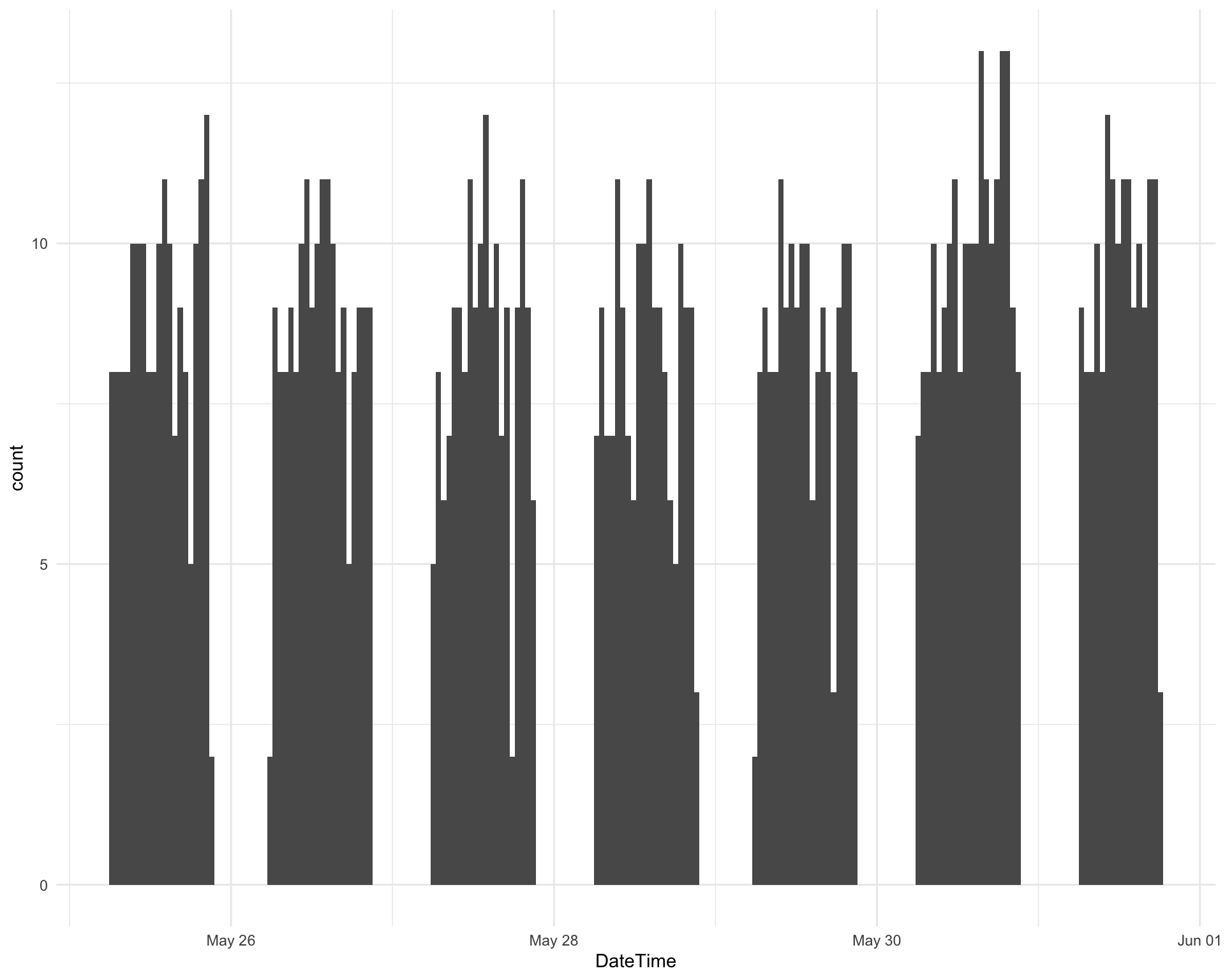

Past versions of DateTime-1.png

Version	Author	Date
8f40292	Luke Zappia	2020-05-31

Chunk time: 0.63 secs

1.2 Song

There are 1128 unique songs. How many times was each song played?

song_counts <- requestival %>%
    group_by(Song, Artist) %>%
    count(name = "PlayCount")

ggplot(song_counts, aes(x = PlayCount)) +
    geom_histogram()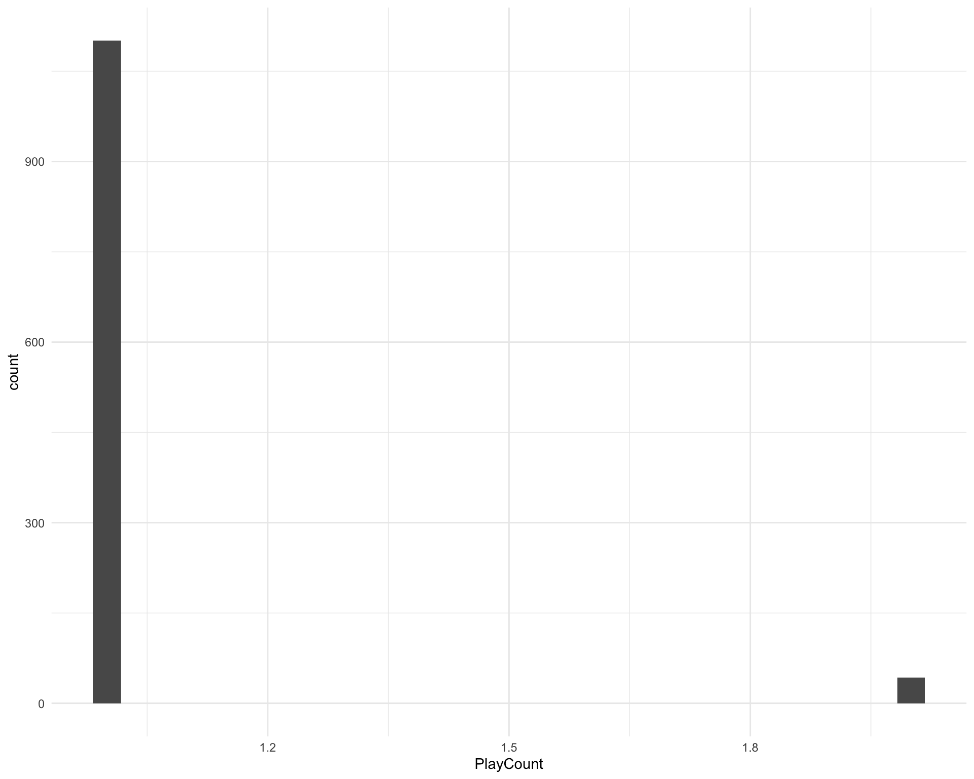

Past versions of Song-count-1.png

Version	Author	Date
8f40292	Luke Zappia	2020-05-31

Chunk time: 0.36 secs

Which songs were played more than once?

song_counts %>%
    filter(PlayCount > 1) %>%
    arrange(-PlayCount)

Chunk time: 0.02 secs

1.3 Artist

There are 896 unique artists. How many times was each artist played?

artist_counts <- requestival %>%
    group_by(Artist) %>%
    count(name = "PlayCount")

ggplot(artist_counts, aes(x = PlayCount)) +
    geom_histogram()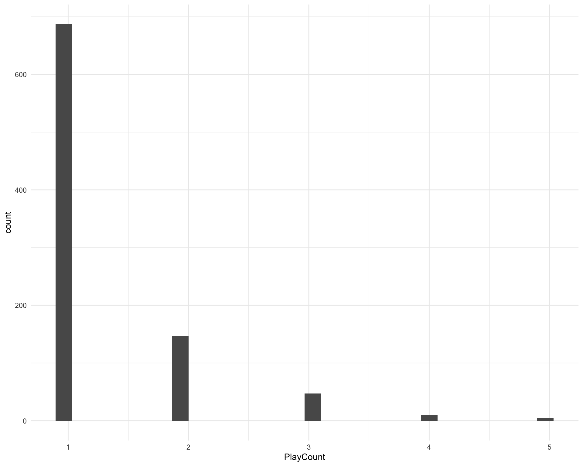

Past versions of Artist-count-1.png

Version	Author	Date
8f40292	Luke Zappia	2020-05-31

Chunk time: 0.27 secs

Which artists were played more than once?

artist_counts %>%
    filter(PlayCount > 1) %>%
    arrange(-PlayCount)

Chunk time: 0.05 secs

1.4 Release

There are 1049 unique releases. How many times was each release played?

release_counts <- requestival %>%
    group_by(Release) %>%
    count(name = "PlayCount")

ggplot(release_counts, aes(x = PlayCount)) +
    geom_histogram()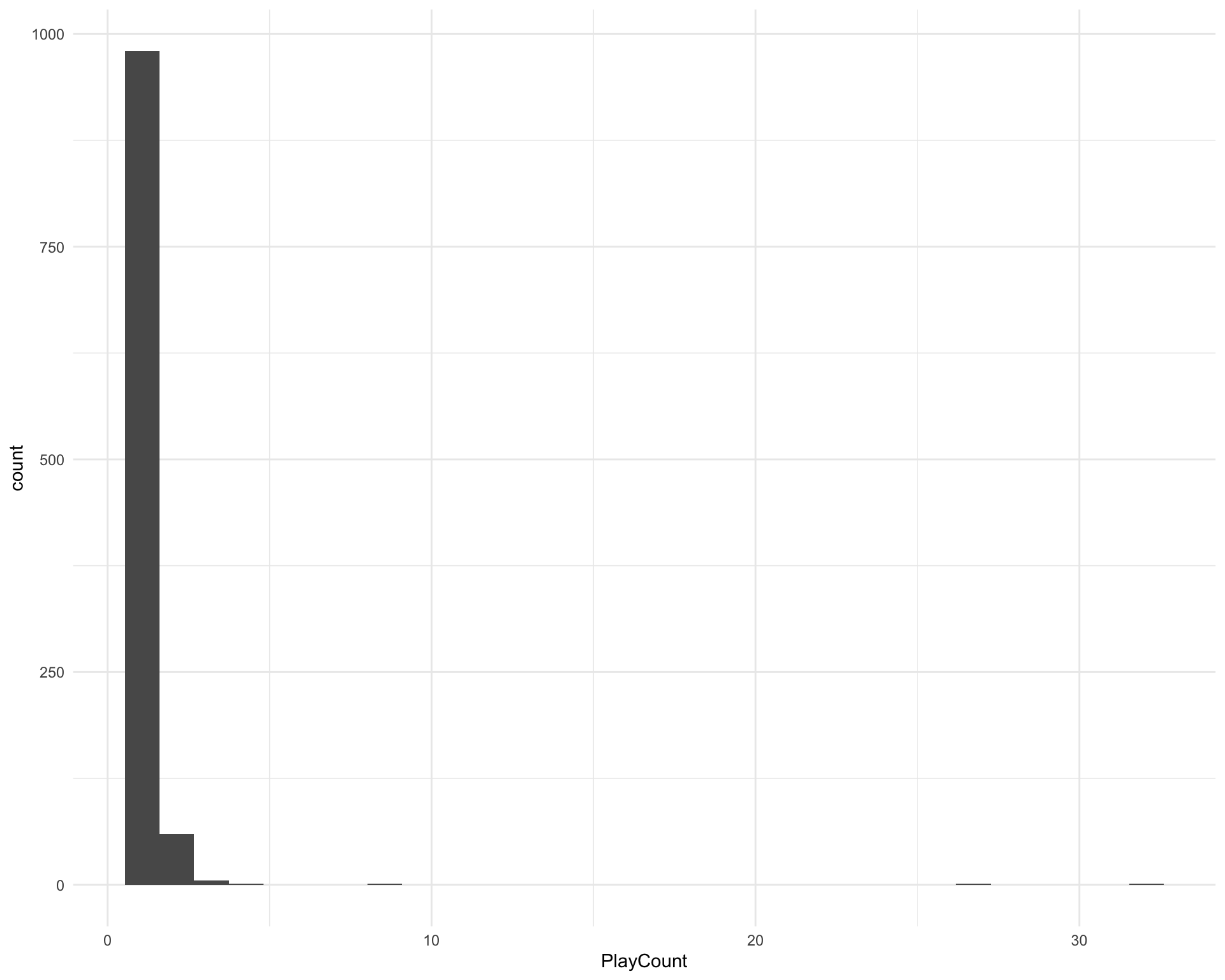

Past versions of Release-count-1.png

Version	Author	Date
8f40292	Luke Zappia	2020-05-31

Chunk time: 0.31 secs

Which releases were played more than once?

release_counts %>%
    filter(PlayCount > 1) %>%
    arrange(-PlayCount)

Chunk time: 0.01 secs

Which songs do not have an associated release?

requestival %>%
    filter(is.na(Release)) %>%
    select(DateTime, Song, Artist)

Chunk time: 0.02 secs

This seems weird but I have checked them and this information is missing from the original HTML pages. It’s only a few songs so I’m not going to try and fix it.

1.5 Unearthed

How many songs are on Unearthed?

ggplot(requestival, aes(x = IsUnearthed)) +
    geom_bar()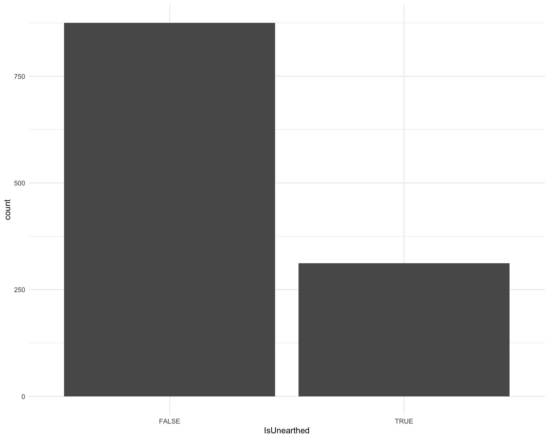

Past versions of Unearthed-1.png

Version	Author	Date
8f40292	Luke Zappia	2020-05-31

Chunk time: 0.26 secs

2 Spotify

Now let’s looks at the fields we downloaded from Spotify. How many songs did we find Spotify track IDs for?

ggplot(requestival, aes(x = HasSpotify)) +
    geom_bar()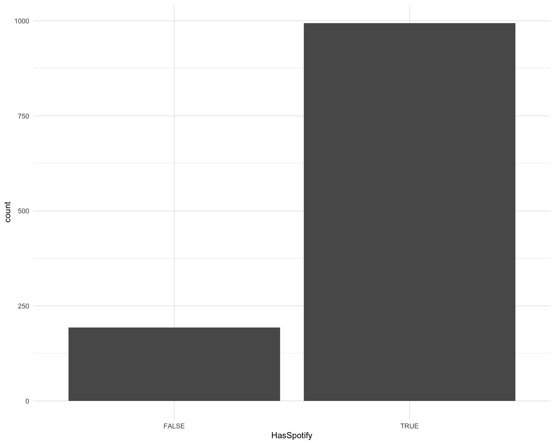

Past versions of HasSpotify-1.png

Version	Author	Date
8f40292	Luke Zappia	2020-05-31

Chunk time: 0.24 secs

For the rest of this section we will only look at the songs with Spotify information.

requestival_spotify <- filter(requestival, HasSpotify)

Chunk time: 0.01 secs

2.1 Album date

When we the songs released? This is the album release date so may not be the earliest song release depending on which album we got from Spotify.

ggplot(requestival_spotify, aes(x = AlbumDate)) +
    geom_histogram()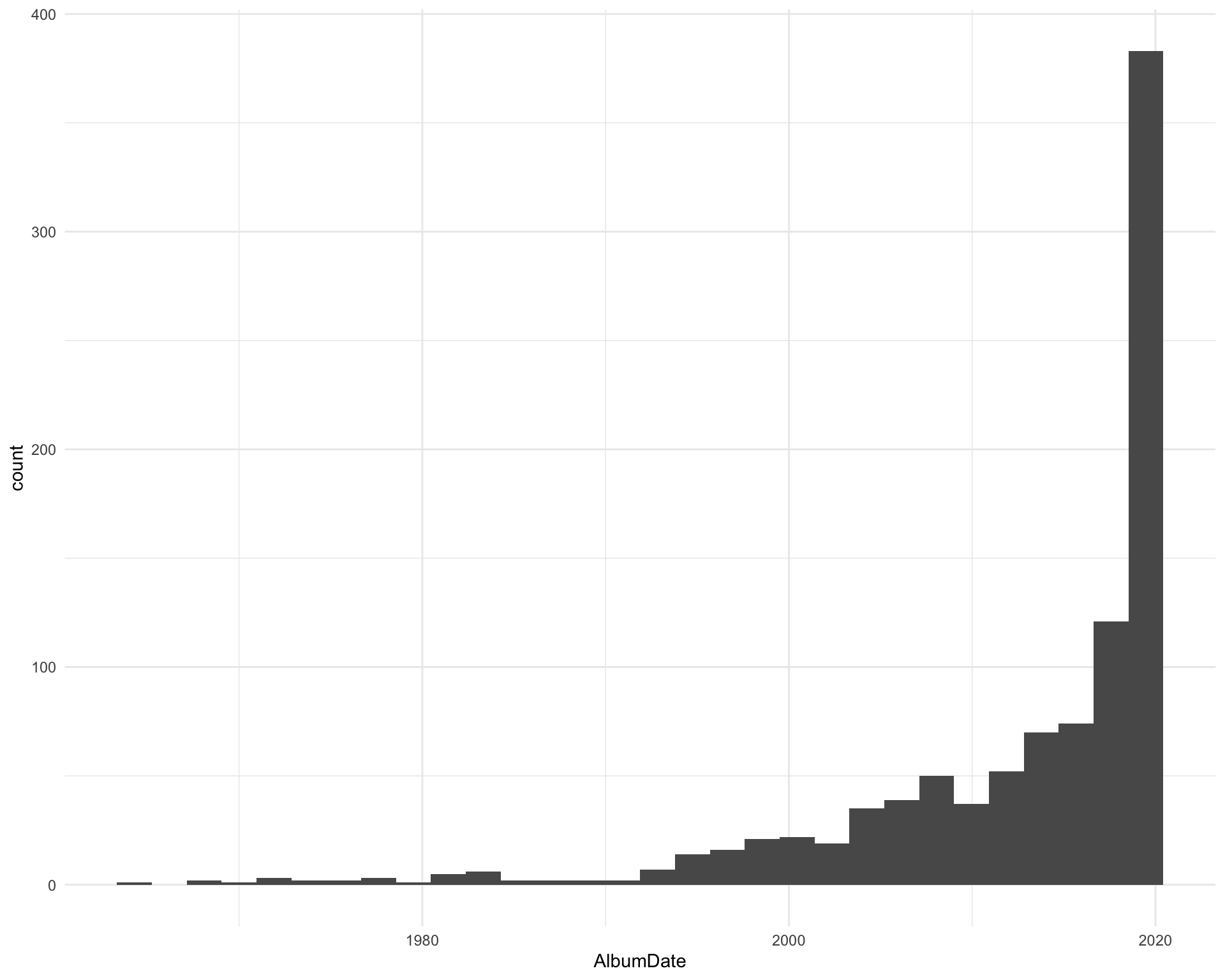

Past versions of AlbumDate-1.png

Version	Author	Date
8f40292	Luke Zappia	2020-05-31

Chunk time: 0.27 secs

The five most recent songs are:

requestival_spotify %>%
    arrange(desc(AlbumDate)) %>%
    top_n(5, AlbumDate) %>%
    select(Song, Artist, Release, AlbumDate)

Chunk time: 0.01 secs

The five oldest songs are:

requestival_spotify %>%
    arrange(AlbumDate) %>%
    top_n(-5, AlbumDate) %>%
    select(Song, Artist, Release, AlbumDate)

Chunk time: 0.31 secs

2.2 Duration

How long are the songs?

ggplot(requestival_spotify, aes(x = Duration)) +
    geom_histogram(bins = 100) +
    scale_x_time()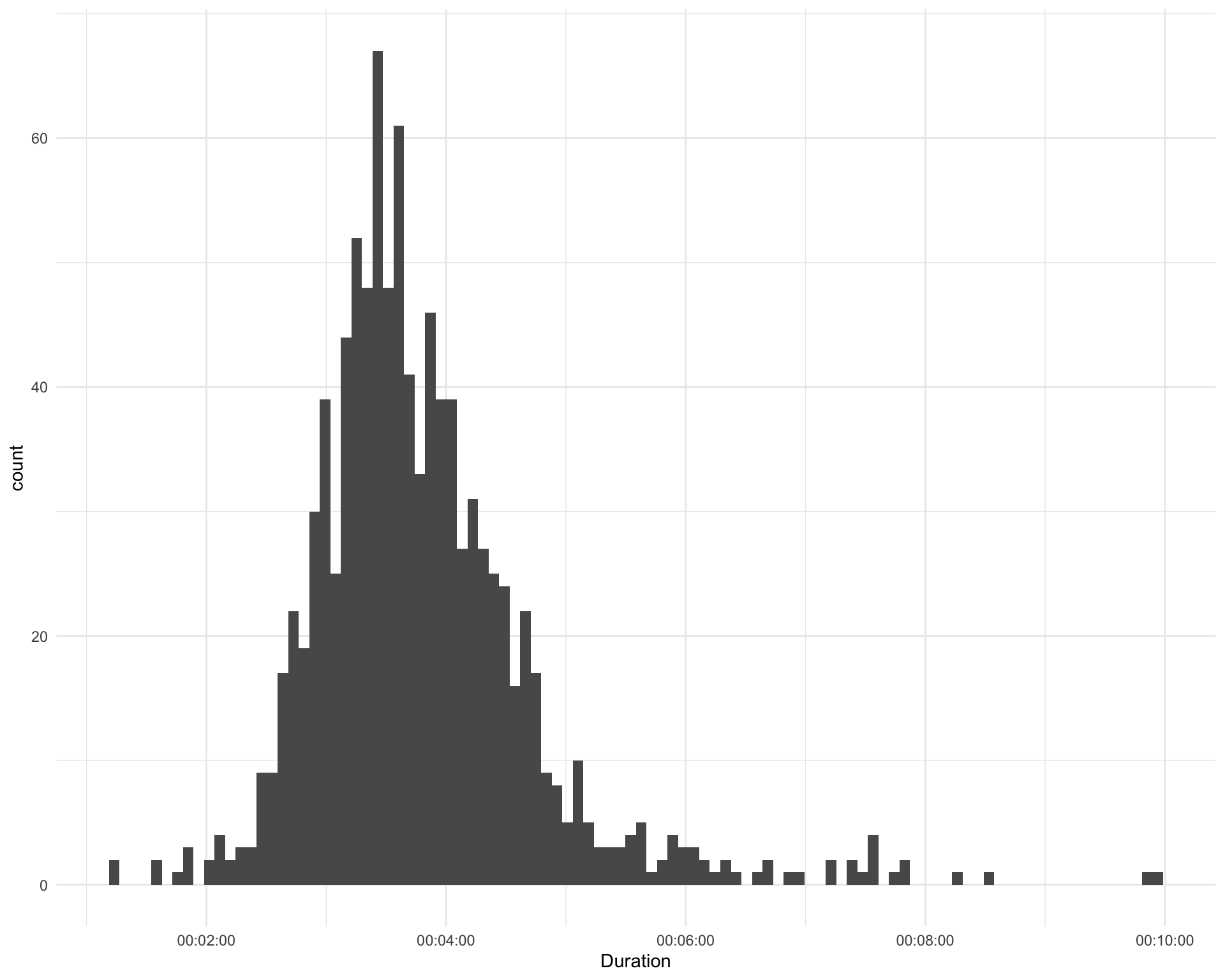

Past versions of Duration-1.png

Version	Author	Date
8f40292	Luke Zappia	2020-05-31

Chunk time: 0.31 secs

The five longest songs are:

requestival_spotify %>%
    arrange(-Duration) %>%
    top_n(5, Duration) %>%
    select(Song, Artist, Duration)

Chunk time: 0.01 secs

The five shortest songs are:

requestival_spotify %>%
    arrange(Duration) %>%
    top_n(-5, Duration) %>%
    select(Song, Artist, Duration)

Chunk time: 0.01 secs

2.3 Explicit

How many songs are explicit?

ggplot(requestival_spotify, aes(x = Explicit)) +
    geom_bar()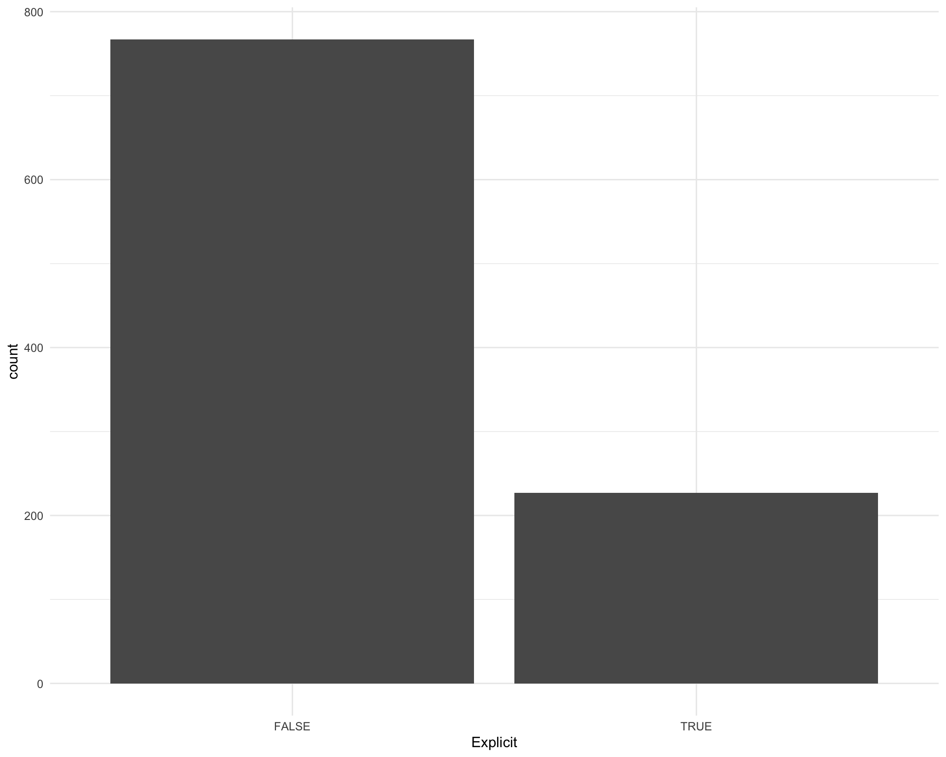

Past versions of Explicit-1.png

Version	Author	Date
8f40292	Luke Zappia	2020-05-31

Chunk time: 0.26 secs

2.4 Popularity

What is the distribution of popularity scores?

ggplot(requestival_spotify, aes(x = Popularity)) +
    geom_bar()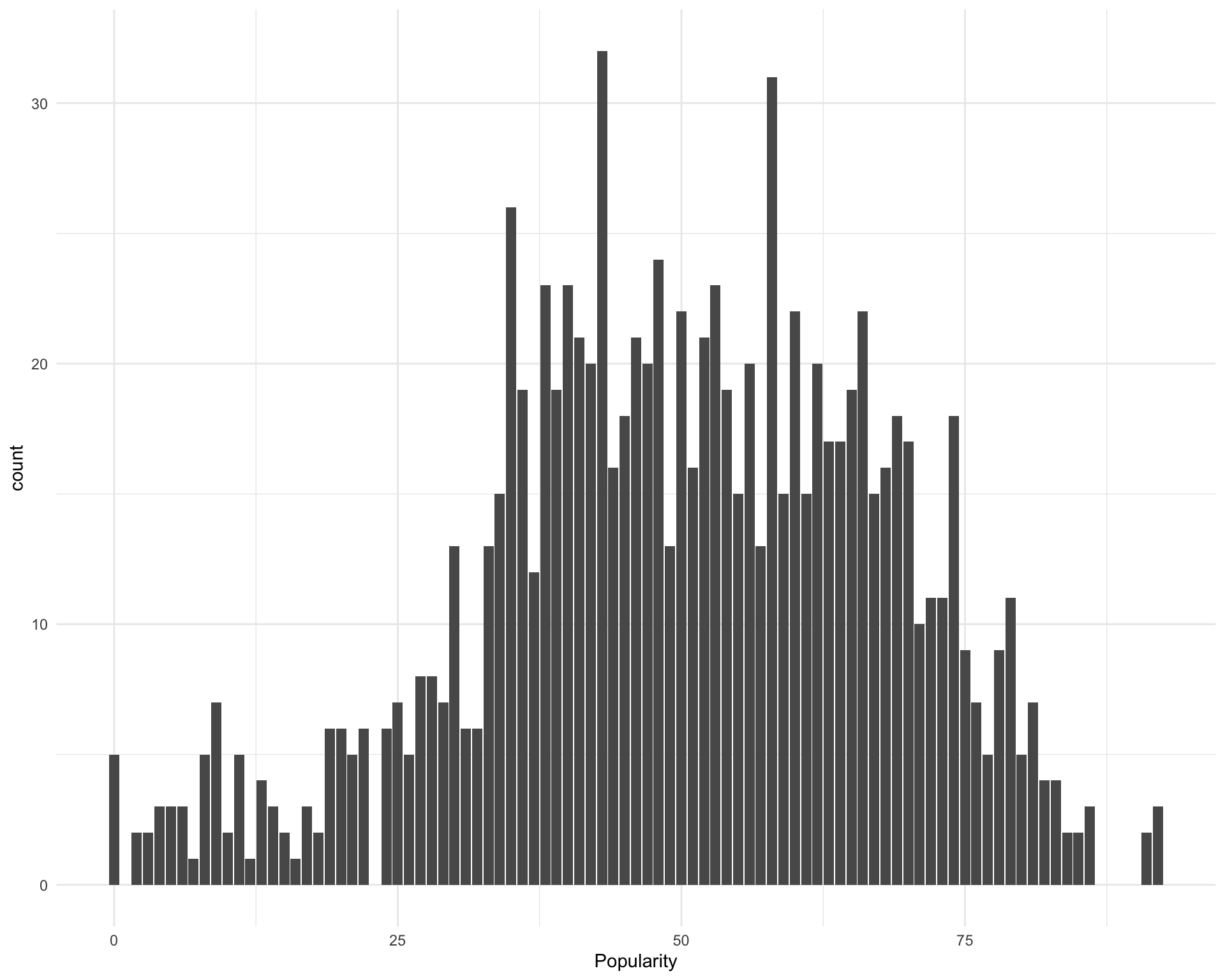

Past versions of Popularity-1.png

Version	Author	Date
8f40292	Luke Zappia	2020-05-31

Chunk time: 0.3 secs

The five most “popular” songs are:

requestival_spotify %>%
    arrange(-Popularity) %>%
    top_n(5, Popularity) %>%
    select(Song, Artist, Popularity)

Chunk time: 0.01 secs

The five least “popular” songs are:

requestival_spotify %>%
    arrange(Popularity) %>%
    top_n(-5, Popularity) %>%
    select(Song, Artist, Popularity)

Chunk time: 0.01 secs

2.5 IsMajor

How many songs are in a major key?

ggplot(requestival_spotify, aes(x = IsMajor)) +
    geom_bar()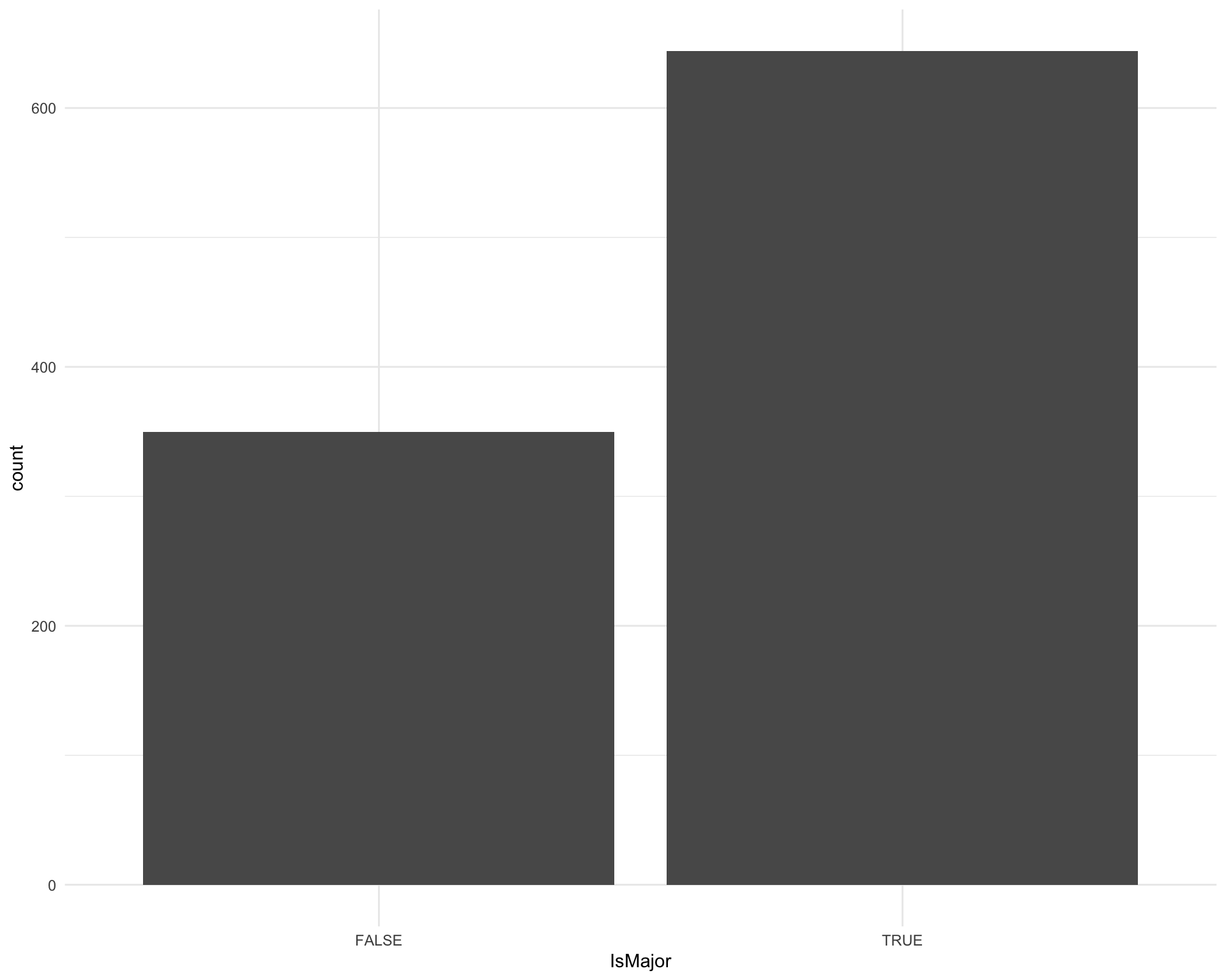

Past versions of IsMajor-1.png

Version	Author	Date
8f40292	Luke Zappia	2020-05-31

Chunk time: 0.23 secs

2.6 Loudness

What is the distribution of loudness?

ggplot(requestival_spotify, aes(x = Loudness)) +
    geom_histogram(bins = 100)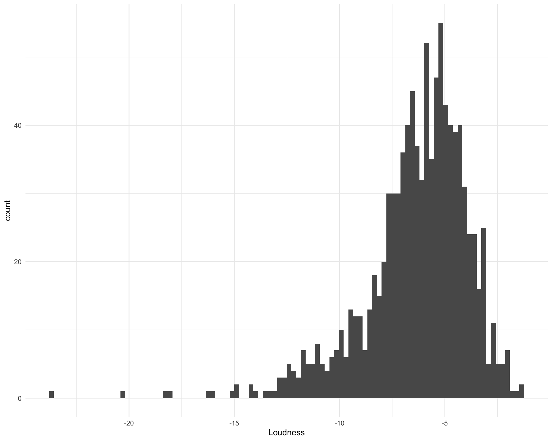

Past versions of Loudness-1.png

Version	Author	Date
8f40292	Luke Zappia	2020-05-31

Chunk time: 0.3 secs

The five loudest songs are:

requestival_spotify %>%
    arrange(-Loudness) %>%
    top_n(5, Loudness) %>%
    select(Song, Artist, Loudness)

Chunk time: 0.01 secs

The five quietest songs are:

requestival_spotify %>%
    arrange(Loudness) %>%
    top_n(-5, Loudness) %>%
    select(Song, Artist, Loudness)

Chunk time: 0.01 secs

2.7 Temp

What speed are the songs?

ggplot(requestival_spotify, aes(x = Tempo)) +
    geom_histogram(bins = 100)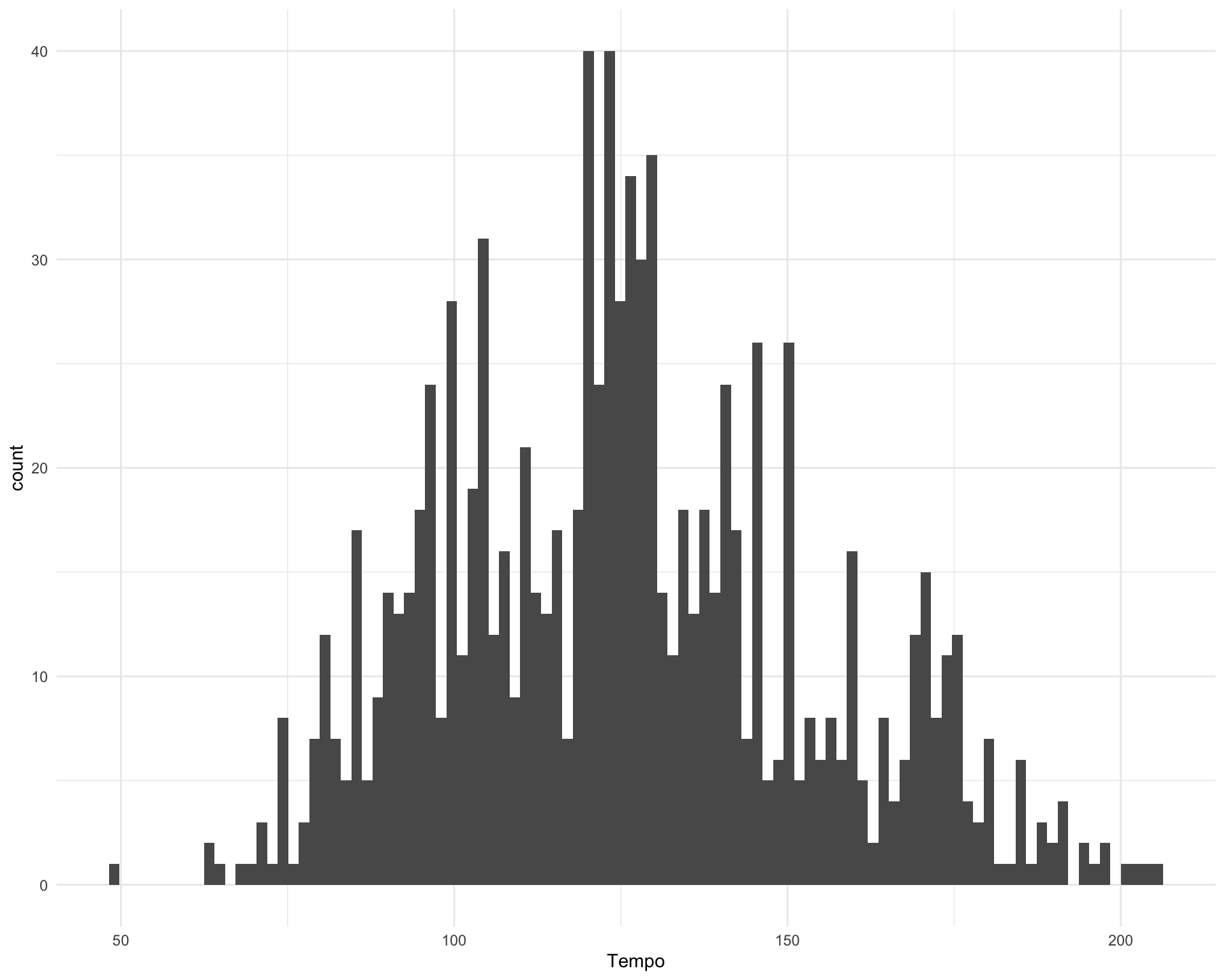

Past versions of Temp-1.png

Version	Author	Date
8f40292	Luke Zappia	2020-05-31

Chunk time: 0.32 secs

The five fastest songs are:

requestival_spotify %>%
    arrange(-Tempo) %>%
    top_n(5, Tempo) %>%
    select(Song, Artist, Tempo)

Chunk time: 0.01 secs

The five slowest songs are:

requestival_spotify %>%
    arrange(Tempo) %>%
    top_n(-5, Tempo) %>%
    select(Song, Artist, Tempo)

Chunk time: 0.01 secs

2.8 Valence

What is the distribution of valence? This is score from zero to one where one is positive and zero is negative.

ggplot(requestival_spotify, aes(x = Valence)) +
    geom_histogram(bins = 100)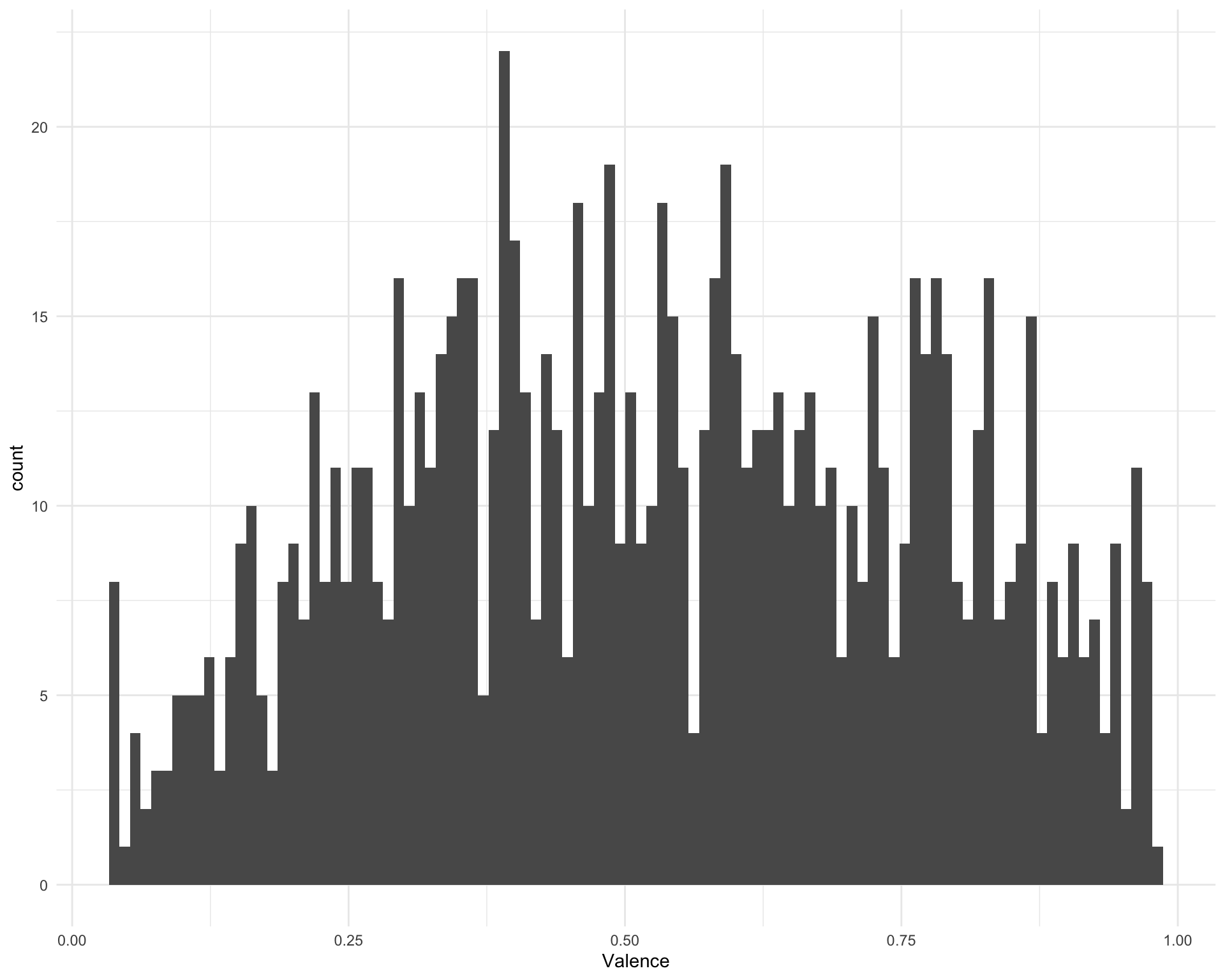

Past versions of Valence-1.png

Version	Author	Date
8f40292	Luke Zappia	2020-05-31

Chunk time: 0.34 secs

The five most positive songs are:

requestival_spotify %>%
    arrange(-Valence) %>%
    top_n(5, Valence) %>%
    select(Song, Artist, Valence)

Chunk time: 0.01 secs

The five most negative songs are:

requestival_spotify %>%
    arrange(Valence) %>%
    top_n(-5, Valence) %>%
    select(Song, Artist, Valence)

Chunk time: 0.01 secs

2.9 Energy

What is the distribution of energy?

ggplot(requestival_spotify, aes(x = Energy)) +
    geom_histogram(bins = 100)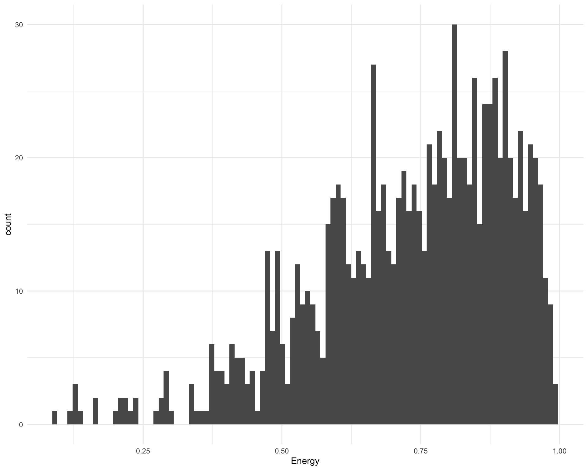

Past versions of Energy-1.png

Version	Author	Date
8f40292	Luke Zappia	2020-05-31

Chunk time: 0.33 secs

The five most energetic songs are:

requestival_spotify %>%
    arrange(-Energy) %>%
    top_n(5, Energy) %>%
    select(Song, Artist, Energy)

Chunk time: 0.01 secs

The five least energetic songs are:

requestival_spotify %>%
    arrange(Energy) %>%
    top_n(-5, Energy) %>%
    select(Song, Artist, Energy)

Chunk time: 0.01 secs

2.10 Danceability

What is the distribution of danceability?

ggplot(requestival_spotify, aes(x = Danceability)) +
    geom_histogram(bins = 100)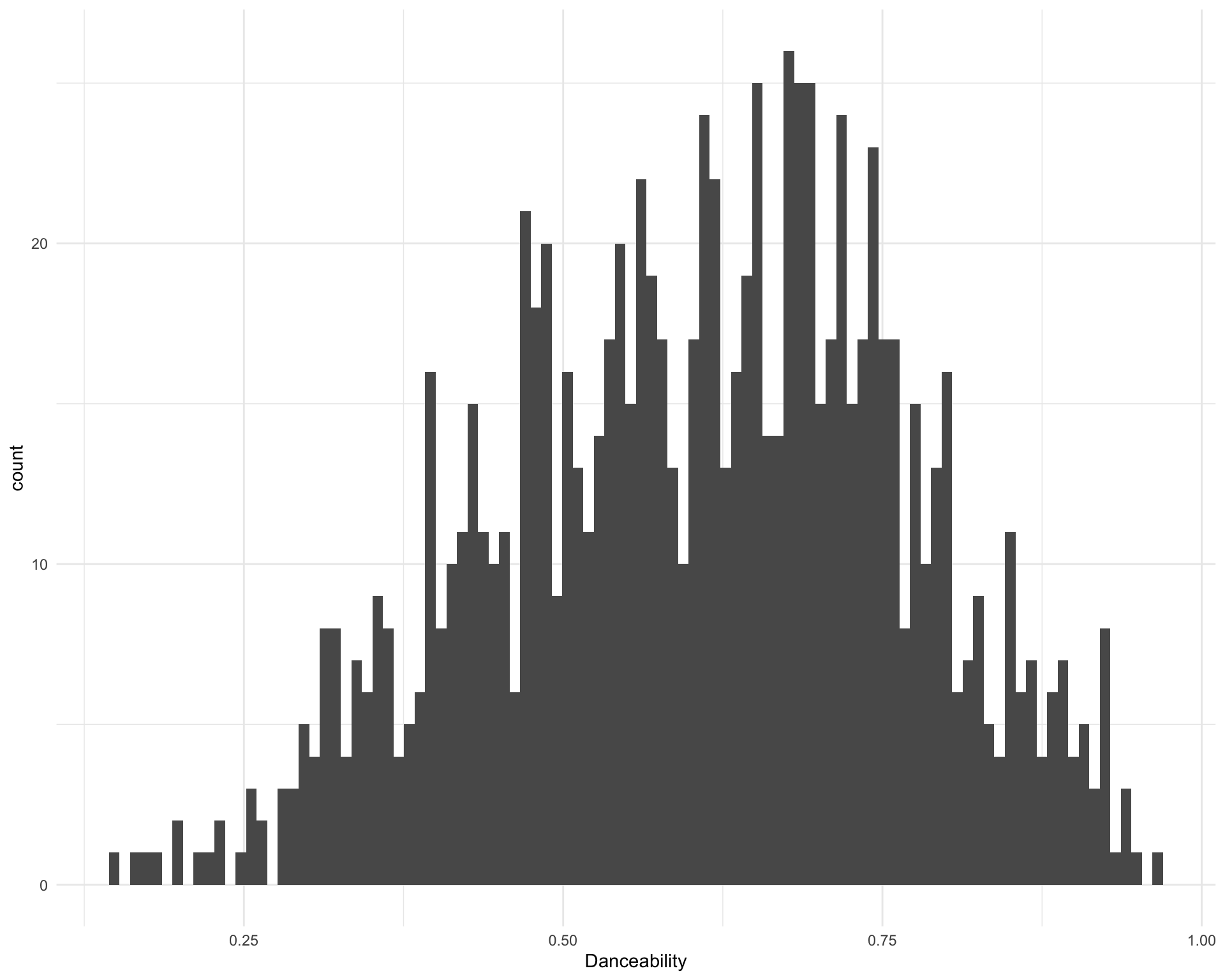

Past versions of Danceability-1.png

Version	Author	Date
8f40292	Luke Zappia	2020-05-31

Chunk time: 0.31 secs

The five most danceable songs are:

requestival_spotify %>%
    arrange(-Danceability) %>%
    top_n(5, Danceability) %>%
    select(Song, Artist, Danceability)

Chunk time: 0.01 secs

The five least danceable songs are:

requestival_spotify %>%
    arrange(Danceability) %>%
    top_n(-5, Danceability) %>%
    select(Song, Artist, Danceability)

Chunk time: 0.01 secs

2.11 Speechiness

What is the distribution of speechiness?

ggplot(requestival_spotify, aes(x = Speechiness)) +
    geom_histogram(bins = 100)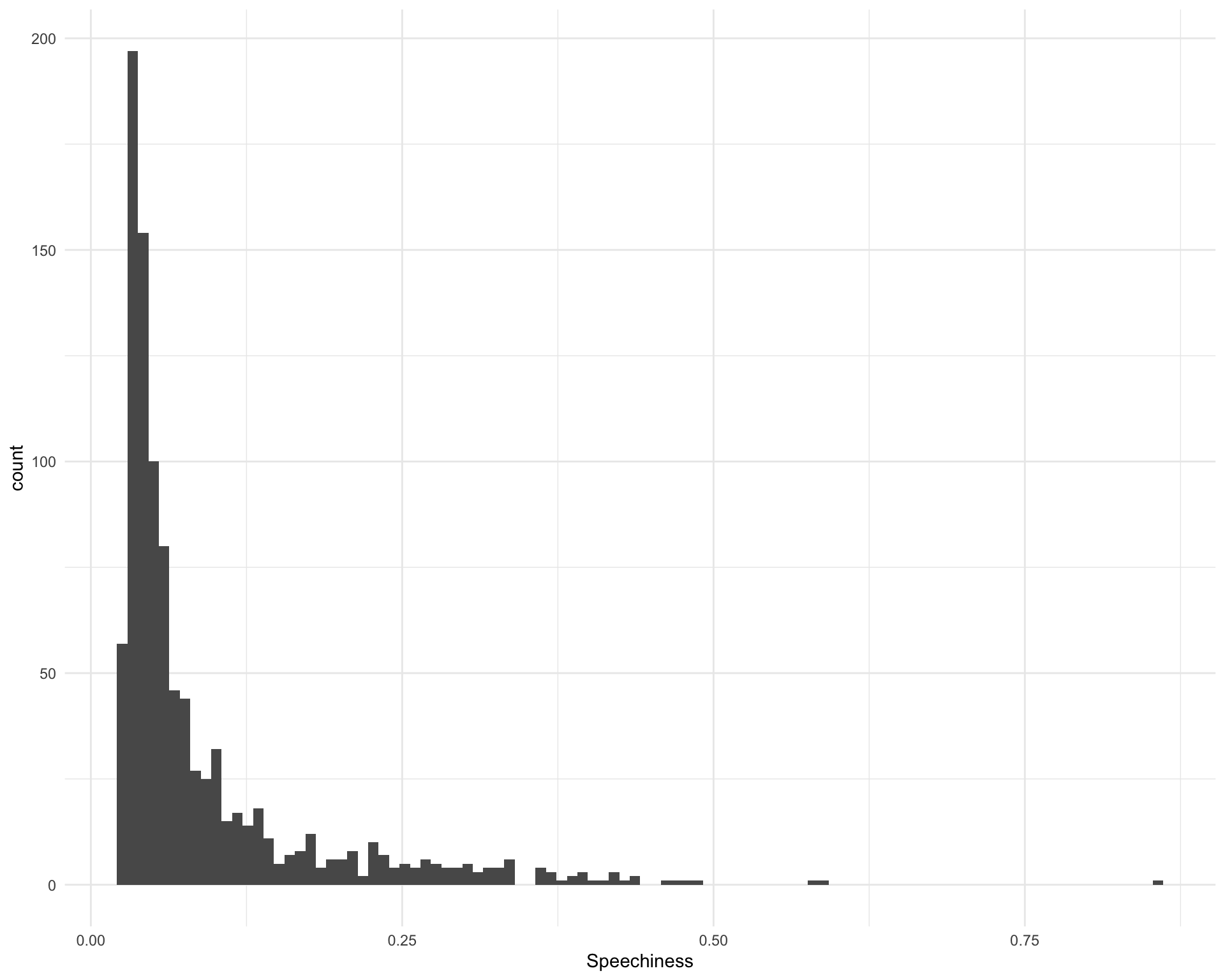

Past versions of Speechiness-1.png

Version	Author	Date
8f40292	Luke Zappia	2020-05-31

Chunk time: 0.32 secs

The five most speechy songs are:

requestival_spotify %>%
    arrange(-Speechiness) %>%
    top_n(5, Speechiness) %>%
    select(Song, Artist, Speechiness)

Chunk time: 0.01 secs

The five least speechy songs are:

requestival_spotify %>%
    arrange(Speechiness) %>%
    top_n(-5, Speechiness) %>%
    select(Song, Artist, Speechiness)

Chunk time: 0.01 secs

2.12 Acousticness

What is the distribution of acousticness?

ggplot(requestival_spotify, aes(x = Acousticness)) +
    geom_histogram(bins = 100)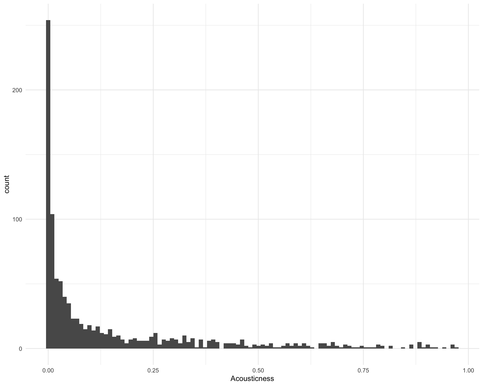

Past versions of Acousticness-1.png

Version	Author	Date
8f40292	Luke Zappia	2020-05-31

Chunk time: 0.33 secs

The five most acoustic songs are:

requestival_spotify %>%
    arrange(-Acousticness) %>%
    top_n(5, Acousticness) %>%
    select(Song, Artist, Acousticness)

Chunk time: 0.01 secs

The five least acoustic are:

requestival_spotify %>%
    arrange(Acousticness) %>%
    top_n(-5, Acousticness) %>%
    select(Song, Artist, Acousticness)

Chunk time: 0.01 secs

2.13 Liveness

What is the distribution of liveness?

ggplot(requestival_spotify, aes(x = Liveness)) +
    geom_histogram(bins = 100)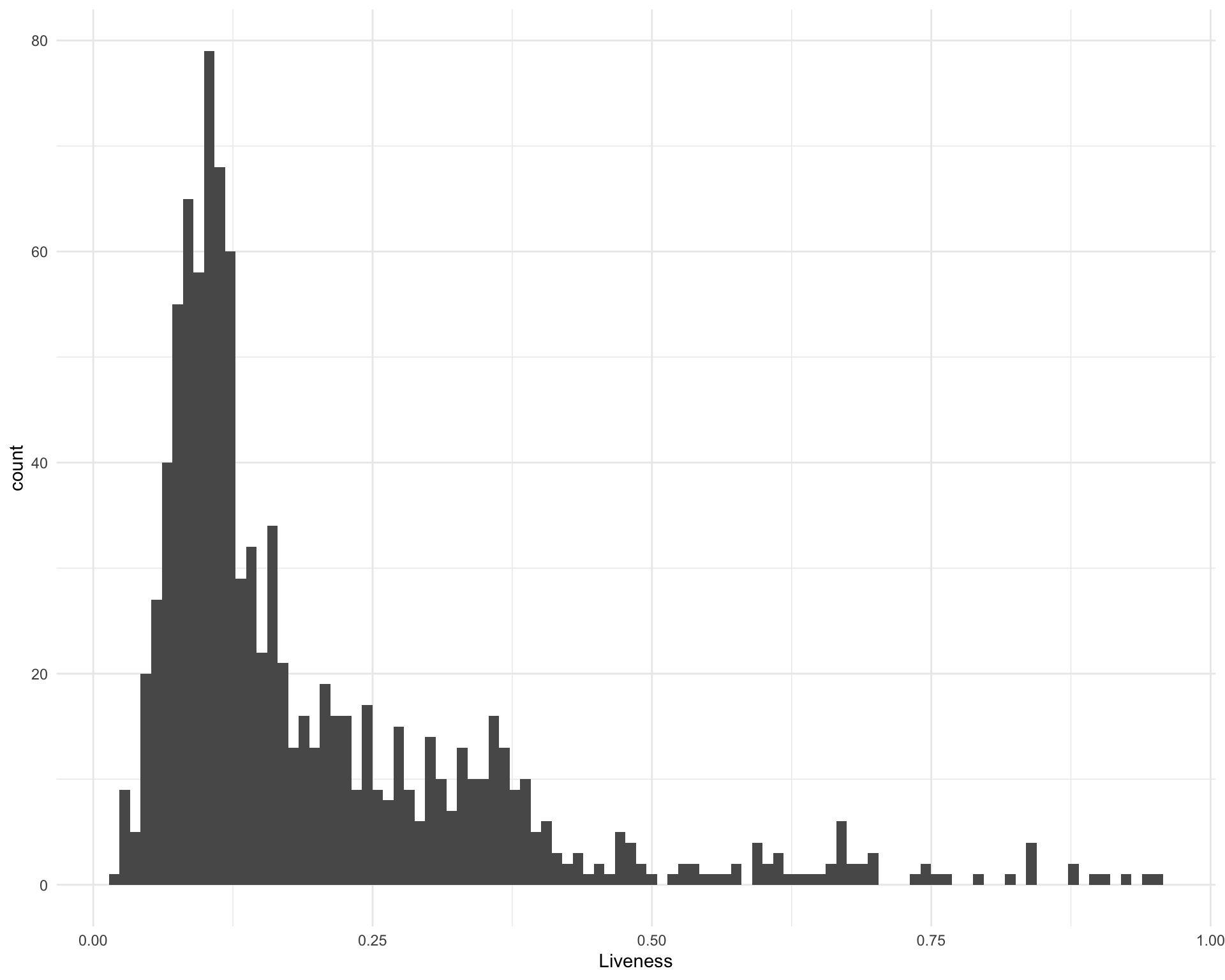

Past versions of Liveness-1.png

Version	Author	Date
8f40292	Luke Zappia	2020-05-31

Chunk time: 0.34 secs

The five most live songs are:

requestival_spotify %>%
    arrange(-Liveness) %>%
    top_n(5, Liveness) %>%
    select(Song, Artist, Liveness)

Chunk time: 0.01 secs

The five least live songs are:

requestival_spotify %>%
    arrange(Liveness) %>%
    top_n(-5, Liveness) %>%
    select(Song, Artist, Liveness)

Chunk time: 0.01 secs

Session information

sessioninfo::session_info()

─ Session info ───────────────────────────────────────────────────────────────
 setting  value                       
 version  R version 4.0.0 (2020-04-24)
 os       macOS Catalina 10.15.4      
 system   x86_64, darwin17.0          
 ui       X11                         
 language (EN)                        
 collate  en_US.UTF-8                 
 ctype    en_US.UTF-8                 
 tz       Europe/Berlin               
 date     2020-06-01                  

─ Packages ───────────────────────────────────────────────────────────────────
 ! package     * version date       lib source           
 P assertthat    0.2.1   2019-03-21 [?] CRAN (R 4.0.0)   
 P backports     1.1.7   2020-05-13 [?] CRAN (R 4.0.0)   
 P base64enc     0.1-3   2015-07-28 [?] CRAN (R 4.0.0)   
 P blob          1.2.1   2020-01-20 [?] CRAN (R 4.0.0)   
 P broom         0.5.6   2020-04-20 [?] CRAN (R 4.0.0)   
 P cellranger    1.1.0   2016-07-27 [?] standard (@1.1.0)
 P cli           2.0.2   2020-02-28 [?] CRAN (R 4.0.0)   
 P colorspace    1.4-1   2019-03-18 [?] standard (@1.4-1)
 P conflicted  * 1.0.4   2019-06-21 [?] standard (@1.0.4)
 P crayon        1.3.4   2017-09-16 [?] CRAN (R 4.0.0)   
 P DBI           1.1.0   2019-12-15 [?] CRAN (R 4.0.0)   
 P dbplyr        1.4.4   2020-05-27 [?] CRAN (R 4.0.0)   
 P digest        0.6.25  2020-02-23 [?] CRAN (R 4.0.0)   
 P dplyr       * 0.8.5   2020-03-07 [?] CRAN (R 4.0.0)   
 P ellipsis      0.3.1   2020-05-15 [?] CRAN (R 4.0.0)   
 P evaluate      0.14    2019-05-28 [?] standard (@0.14) 
 P fansi         0.4.1   2020-01-08 [?] CRAN (R 4.0.0)   
 P farver        2.0.3   2020-01-16 [?] CRAN (R 4.0.0)   
 P forcats     * 0.5.0   2020-03-01 [?] CRAN (R 4.0.0)   
 P fs          * 1.4.1   2020-04-04 [?] CRAN (R 4.0.0)   
 P generics      0.0.2   2018-11-29 [?] standard (@0.0.2)
 P genius        2.2.2   2020-05-28 [?] CRAN (R 4.0.0)   
 P ggplot2     * 3.3.1   2020-05-28 [?] CRAN (R 4.0.0)   
 P git2r         0.27.1  2020-05-03 [?] CRAN (R 4.0.0)   
 P glue        * 1.4.1   2020-05-13 [?] CRAN (R 4.0.0)   
 P gtable        0.3.0   2019-03-25 [?] standard (@0.3.0)
 P haven         2.3.0   2020-05-24 [?] CRAN (R 4.0.0)   
 P here        * 0.1     2017-05-28 [?] standard (@0.1)  
 P hms           0.5.3   2020-01-08 [?] CRAN (R 4.0.0)   
 P htmltools     0.4.0   2019-10-04 [?] standard (@0.4.0)
 P httpuv        1.5.3.1 2020-05-26 [?] CRAN (R 4.0.0)   
 P httr          1.4.1   2019-08-05 [?] standard (@1.4.1)
 P janeaustenr   0.1.5   2017-06-10 [?] CRAN (R 4.0.0)   
 P jsonlite      1.6.1   2020-02-02 [?] CRAN (R 4.0.0)   
 P knitr         1.28    2020-02-06 [?] CRAN (R 4.0.0)   
 P labeling      0.3     2014-08-23 [?] standard (@0.3)  
 P later         1.0.0   2019-10-04 [?] standard (@1.0.0)
 P lattice       0.20-41 2020-04-02 [3] CRAN (R 4.0.0)   
 P lifecycle     0.2.0   2020-03-06 [?] CRAN (R 4.0.0)   
 P lubridate   * 1.7.8   2020-04-06 [?] CRAN (R 4.0.0)   
 P magrittr      1.5     2014-11-22 [?] CRAN (R 4.0.0)   
 P Matrix        1.2-18  2019-11-27 [3] CRAN (R 4.0.0)   
 P memoise       1.1.0   2017-04-21 [?] standard (@1.1.0)
 P modelr        0.1.8   2020-05-19 [?] CRAN (R 4.0.0)   
 P munsell       0.5.0   2018-06-12 [?] standard (@0.5.0)
 P nlme          3.1-147 2020-04-13 [3] CRAN (R 4.0.0)   
 P pillar        1.4.4   2020-05-05 [?] CRAN (R 4.0.0)   
 P pkgconfig     2.0.3   2019-09-22 [?] CRAN (R 4.0.0)   
 P plyr          1.8.6   2020-03-03 [?] CRAN (R 4.0.0)   
 P promises      1.1.0   2019-10-04 [?] standard (@1.1.0)
 P purrr       * 0.3.4   2020-04-17 [?] CRAN (R 4.0.0)   
 P R6            2.4.1   2019-11-12 [?] CRAN (R 4.0.0)   
 P Rcpp          1.0.4.6 2020-04-09 [?] CRAN (R 4.0.0)   
 P readr       * 1.3.1   2018-12-21 [?] standard (@1.3.1)
 P readxl        1.3.1   2019-03-13 [?] standard (@1.3.1)
 P reprex        0.3.0   2019-05-16 [?] standard (@0.3.0)
 P reshape2      1.4.4   2020-04-09 [?] CRAN (R 4.0.0)   
 P rlang         0.4.6   2020-05-02 [?] CRAN (R 4.0.0)   
 P rmarkdown     2.1     2020-01-20 [?] CRAN (R 4.0.0)   
 P rprojroot     1.3-2   2018-01-03 [?] CRAN (R 4.0.0)   
 P rstudioapi    0.11    2020-02-07 [?] CRAN (R 4.0.0)   
 P rvest       * 0.3.5   2019-11-08 [?] standard (@0.3.5)
 P scales        1.1.1   2020-05-11 [?] CRAN (R 4.0.0)   
   sessioninfo   1.1.1   2018-11-05 [3] CRAN (R 4.0.0)   
 P SnowballC     0.7.0   2020-04-01 [?] CRAN (R 4.0.0)   
 P spotifyr    * 2.1.1   2019-07-13 [?] CRAN (R 4.0.0)   
 P stringi       1.4.6   2020-02-17 [?] CRAN (R 4.0.0)   
 P stringr     * 1.4.0   2019-02-10 [?] CRAN (R 4.0.0)   
 P tibble      * 3.0.1   2020-04-20 [?] CRAN (R 4.0.0)   
 P tidyr       * 1.1.0   2020-05-20 [?] CRAN (R 4.0.0)   
 P tidyselect    1.1.0   2020-05-11 [?] CRAN (R 4.0.0)   
 P tidytext      0.2.4   2020-04-17 [?] CRAN (R 4.0.0)   
 P tidyverse   * 1.3.0   2019-11-21 [?] standard (@1.3.0)
 P tokenizers    0.2.1   2018-03-29 [?] CRAN (R 4.0.0)   
 P vctrs         0.3.0   2020-05-11 [?] CRAN (R 4.0.0)   
 P whisker       0.4     2019-08-28 [?] standard (@0.4)  
 P withr         2.2.0   2020-04-20 [?] CRAN (R 4.0.0)   
 P workflowr     1.6.2   2020-04-30 [?] CRAN (R 4.0.0)   
 P xfun          0.14    2020-05-20 [?] CRAN (R 4.0.0)   
 P xml2        * 1.3.2   2020-04-23 [?] CRAN (R 4.0.0)   
 P yaml          2.2.1   2020-02-01 [?] CRAN (R 4.0.0)   

[1] /Users/luke.zappia/Documents/Projects/requestival/renv/library/R-4.0/x86_64-apple-darwin17.0
[2] /private/var/folders/rj/60lhr791617422kqvh0r4vy40000gn/T/RtmpQWp4dI/renv-system-library
[3] /Library/Frameworks/R.framework/Versions/4.0/Resources/library

 P ── Loaded and on-disk path mismatch.

Chunk time: 0.2 secs