Plot a clustering tree — clustree • clustree

Creates a plot of a clustering tree showing the relationship between clusterings at different resolutions.

Usage

clustree(x, ...)

# S3 method for matrix
clustree(
  x,
  prefix,
  suffix = NULL,
  metadata = NULL,
  count_filter = 0,
  prop_filter = 0.1,
  layout = c("tree", "sugiyama"),
  use_core_edges = TRUE,
  highlight_core = FALSE,
  node_colour = prefix,
  node_colour_aggr = NULL,
  node_size = "size",
  node_size_aggr = NULL,
  node_size_range = c(4, 15),
  node_alpha = 1,
  node_alpha_aggr = NULL,
  node_text_size = 3,
  scale_node_text = FALSE,
  node_text_colour = "black",
  node_text_angle = 0,
  node_label = NULL,
  node_label_aggr = NULL,
  node_label_size = 3,
  node_label_nudge = -0.2,
  edge_width = 1.5,
  edge_arrow = TRUE,
  edge_arrow_ends = c("last", "first", "both"),
  show_axis = FALSE,
  return = c("plot", "graph", "layout"),
  ...
)

# S3 method for data.frame
clustree(x, prefix, ...)

# S3 method for SingleCellExperiment
clustree(x, prefix, exprs = "counts", ...)

# S3 method for seurat
clustree(x, prefix = "res.", exprs = c("data", "raw.data", "scale.data"), ...)

# S3 method for Seurat
clustree(
  x,
  prefix = paste0(assay, "_snn_res."),
  exprs = c("data", "counts", "scale.data"),
  assay = NULL,
  ...
)

Arguments

x: object containing clustering data
...: extra parameters passed to other methods
prefix: string indicating columns containing clustering information
suffix: string at the end of column names containing clustering information
metadata: data.frame containing metadata on each sample that can be used as node aesthetics
count_filter: count threshold for filtering edges in the clustering graph
prop_filter: in proportion threshold for filtering edges in the clustering graph
layout: string specifying the "tree" or "sugiyama" layout, see igraph::layout_as_tree() and igraph::layout_with_sugiyama() for details
use_core_edges: logical, whether to only use core tree (edges with maximum in proportion for a node) when creating the graph layout, all (unfiltered) edges will still be displayed
highlight_core: logical, whether to increase the edge width of the core network to make it easier to see
node_colour: either a value indicating a colour to use for all nodes or the name of a metadata column to colour nodes by
node_colour_aggr: if node_colour is a column name than a string giving the name of a function to aggregate that column for samples in each cluster
node_size: either a numeric value giving the size of all nodes or the name of a metadata column to use for node sizes
node_size_aggr: if node_size is a column name than a string giving the name of a function to aggregate that column for samples in each cluster
node_size_range: numeric vector of length two giving the maximum and minimum point size for plotting nodes
node_alpha: either a numeric value giving the alpha of all nodes or the name of a metadata column to use for node transparency
node_alpha_aggr: if node_aggr is a column name than a string giving the name of a function to aggregate that column for samples in each cluster
node_text_size: numeric value giving the size of node text if scale_node_text is FALSE
scale_node_text: logical indicating whether to scale node text along with the node size
node_text_colour: colour value for node text (and label)
node_text_angle: the rotation of the node text
node_label: additional label to add to nodes
node_label_aggr: if node_label is a column name than a string giving the name of a function to aggregate that column for samples in each cluster
node_label_size: numeric value giving the size of node label text
node_label_nudge: numeric value giving nudge in y direction for node labels
edge_width: numeric value giving the width of plotted edges
edge_arrow: logical indicating whether to add an arrow to edges
edge_arrow_ends: string indicating which ends of the line to draw arrow heads if edge_arrow is TRUE, one of "last", "first", or "both"
show_axis: whether to show resolution axis
return: string specifying what to return, either "plot" (a ggplot object), "graph" (a tbl_graph object) or "layout" (a ggraph layout object)
exprs: source of gene expression information to use as node aesthetics, for SingleCellExperiment objects it must be a name in assayNames(x), for a seurat object it must be one of data, raw.data or scale.data and for a Seurat object it must be one of data, counts or scale.data
assay: name of assay to pull expression and clustering data from for Seurat objects

Value

a ggplot object (default), a tbl_graph object or a ggraph

layout object depending on the value of return

Details

Data sources

Plotting a clustering tree requires information about which cluster each sample has been assigned to at different resolutions. This information can be supplied in various forms, as a matrix, data.frame or more specialised object. In all cases the object provided must contain numeric columns with the naming structure PXS where P is a prefix indicating that the column contains clustering information, X is a numeric value indicating the clustering resolution and S is any additional suffix to be removed. For SingleCellExperiment objects this information must be in the colData slot and for Seurat objects it must be in the meta.data slot. For all objects except matrices any additional columns can be used as aesthetics, for matrices an additional metadata data.frame can be supplied if required.

Filtering

Edges in the graph can be filtered by adjusting the count_filter and prop_filter parameters. The count_filter removes any edges that represent less than that number of samples, while the prop_filter removes edges that represent less than that proportion of cells in the node it points towards.

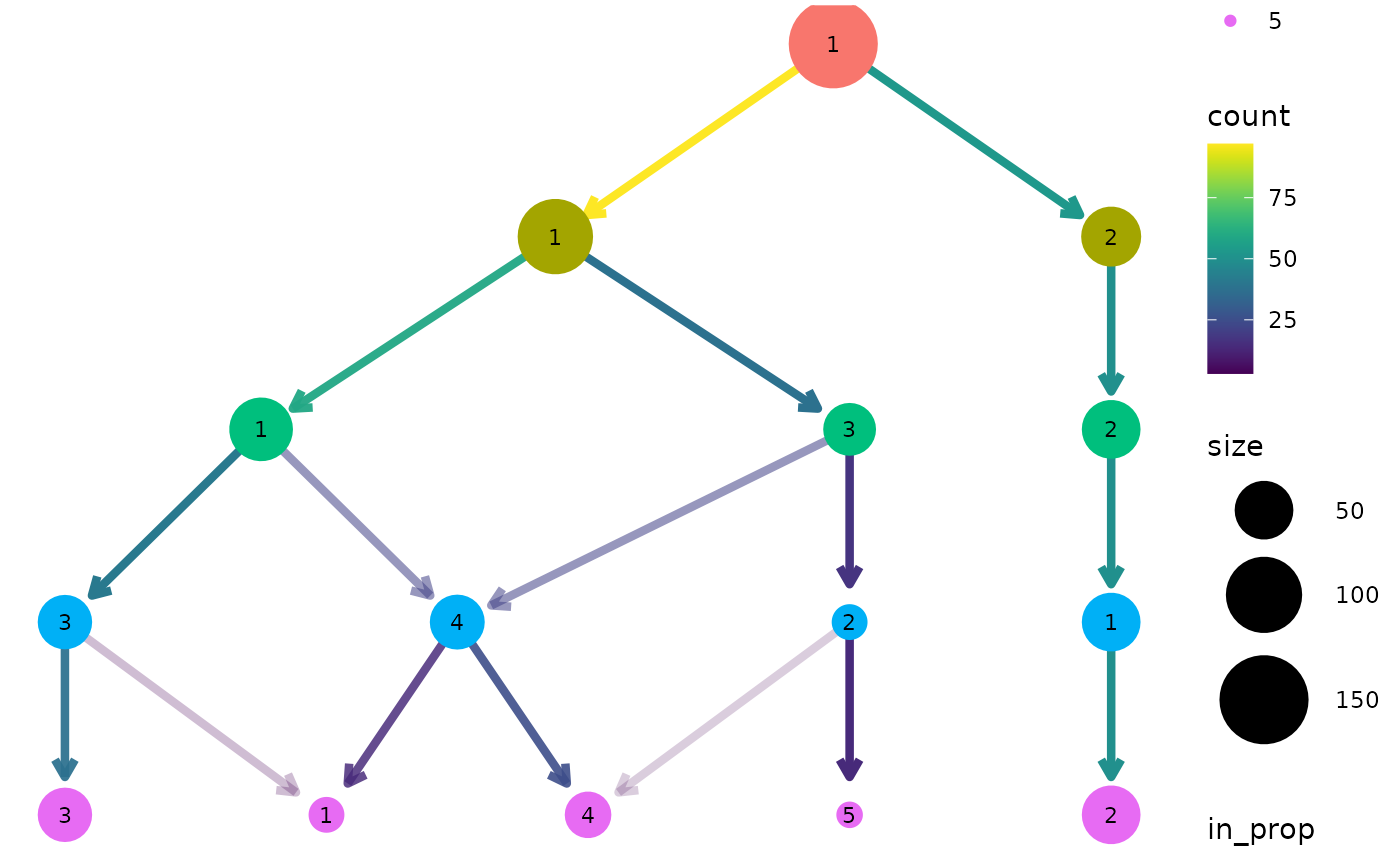
Node aesthetics

The aesthetics of the plotted nodes can be controlled in various ways. By default the colour indicates the clustering resolution, the size indicates the number of samples in that cluster and the transparency is set to 100%. Each of these can be set to a specific value or linked to a supplied metadata column. For a SingleCellExperiment or Seurat object the names of genes can also be used. If a metadata column is used than an aggregation function must also be supplied to combine the samples in each cluster. This function must take a vector of values and return a single value.

Layout

The clustering tree can be displayed using either the Reingold-Tilford tree layout algorithm or the Sugiyama layout algorithm for layered directed acyclic graphs. These layouts were selected as the are the algorithms available in the igraph package designed for trees. The Reingold-Tilford algorithm places children below their parents while the Sugiyama places nodes in layers while trying to minimise the number of crossing edges. See igraph::layout_as_tree() and igraph::layout_with_sugiyama() for more details. When use_core_edges is TRUE (default) only the core tree of the maximum in proportion edges for each node are used for constructing the layout. This can often lead to more attractive layouts where the core tree is more visible.

Examples

data(nba_clusts)
clustree(nba_clusts, prefix = "K")