Last updated: 2019-06-26

Checks: 7 0

Knit directory: OzSingleCells2019/

This reproducible R Markdown analysis was created with workflowr (version 1.4.0). The Checks tab describes the reproducibility checks that were applied when the results were created. The Past versions tab lists the development history.

R Markdown file: up-to-date

Great! Since the R Markdown file has been committed to the Git repository, you know the exact version of the code that produced these results.

Environment: empty

Great job! The global environment was empty. Objects defined in the global environment can affect the analysis in your R Markdown file in unknown ways. For reproduciblity it’s best to always run the code in an empty environment.

Seed: set.seed(20190619)

The command set.seed(20190619) was run prior to running the code in the R Markdown file. Setting a seed ensures that any results that rely on randomness, e.g. subsampling or permutations, are reproducible.

Session information: recorded

Great job! Recording the operating system, R version, and package versions is critical for reproducibility.

Cache: none

Nice! There were no cached chunks for this analysis, so you can be confident that you successfully produced the results during this run.

File paths: relative

Great job! Using relative paths to the files within your workflowr project makes it easier to run your code on other machines.

Repository version: 8627b5b

Great! You are using Git for version control. Tracking code development and connecting the code version to the results is critical for reproducibility. The version displayed above was the version of the Git repository at the time these results were generated.

Note that you need to be careful to ensure that all relevant files for the analysis have been committed to Git prior to generating the results (you can use wflow_publish or wflow_git_commit). workflowr only checks the R Markdown file, but you know if there are other scripts or data files that it depends on. Below is the status of the Git repository when the results were generated:


Ignored files:
    Ignored:    .DS_Store
    Ignored:    .Rhistory
    Ignored:    .Rproj.user/
    Ignored:    ._.DS_Store
    Ignored:    analysis/cache/
    Ignored:    data/._antibody_genes.tsv
    Ignored:    data/._antibody_genes.txt
    Ignored:    docs/.DS_Store
    Ignored:    docs/._.DS_Store
    Ignored:    output/03-comparison.Rmd/
    Ignored:    packrat/lib-R/
    Ignored:    packrat/lib-ext/
    Ignored:    packrat/lib/
    Ignored:    packrat/src/

Untracked files:
    Untracked:  analysis/05-cite-clustering.Rmd

Unstaged changes:
    Modified:   R/set_paths.R
    Modified:   data/02-CITE-filtered.Rds
    Modified:   data/02-filtered.Rds
    Modified:   output/02-quality-control.Rmd/parameters.json

Note that any generated files, e.g. HTML, png, CSS, etc., are not included in this status report because it is ok for generated content to have uncommitted changes.

These are the previous versions of the R Markdown and HTML files. If you’ve configured a remote Git repository (see ?wflow_git_remote), click on the hyperlinks in the table below to view them.

File	Version	Author	Date	Message
Rmd	8627b5b	Luke Zappia	2019-06-26	Remove all zero CITE cells
html	c602800	Luke Zappia	2019-06-20	Add quality control

#### LIBRARIES ####
# Package conflicts
library("conflicted")

# Single-cell
library("SingleCellExperiment")
library("scater")

# RNA-seq
library("edgeR")

# File paths
library("fs")
library("here")

# Presentation
library("knitr")
library("jsonlite")
library("cowplot")

# Tidyverse
library("tidyverse")

### CONFLICT PREFERENCES ####
conflict_prefer("path", "fs")
conflict_prefer("mutate", "dplyr")
conflict_prefer("arrange", "dplyr") 

### SOURCE FUNCTIONS ####
source(here("R/output.R"))
source(here("R/plotting.R"))

### OUTPUT DIRECTORY ####
OUT_DIR <- here("output", DOCNAME)
dir_create(OUT_DIR)

#### SET GGPLOT THEME ####
theme_set(theme_minimal())

#### SET PATHS ####
source(here("R/set_paths.R"))

Introduction

In this document we are going to load perform quality control of the RNA-seq dataset.

if (all(file_exists(c(PATHS$sce_sel, PATHS$cite_sel)))) {
    sce <- read_rds(PATHS$sce_sel)
    cite <- read_rds(PATHS$cite_sel)
} else {
    stop("Selected dataset is missing. ",
         "Please run '01-pre-processing.Rmd' first.",
         call. = FALSE)
}

set.seed(1)
sizeFactors(sce) <- librarySizeFactors(sce)
sce <- normalize(sce)
sce <- runPCA(sce)
sce <- runTSNE(sce)
#sce <- runUMAP(sce)
col_data <- as.data.frame(colData(sce))
row_data <- as.data.frame(rowData(sce))

Exploration

We will start off by making some plots to explore the dataset.

Expression by cell

Distributions by cell. Blue line shows the median and red lines show median absolute deviations (MADs) from the median.

Total counts

outlier_histogram(col_data, "log10_total_counts", mads = 1:6)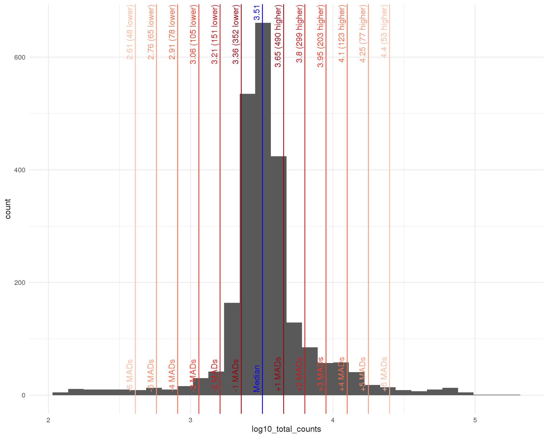

Version	Author	Date
c602800	Luke Zappia	2019-06-20

Total features

outlier_histogram(col_data, "log10_total_features_by_counts", mads = 1:6)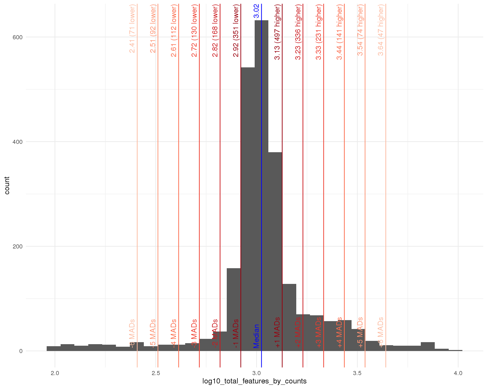

Version	Author	Date
c602800	Luke Zappia	2019-06-20

Percent mitochondrial

outlier_histogram(col_data, "pct_counts_MT", mads = c(1, 3, 5, 7))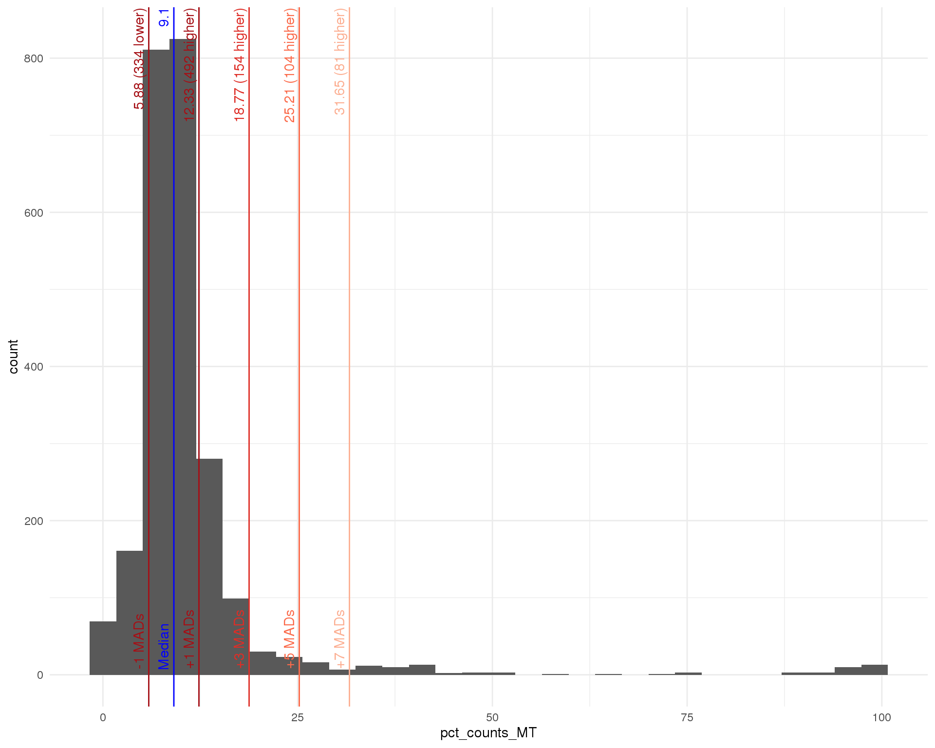

Version	Author	Date
c602800	Luke Zappia	2019-06-20

Dimensionality reduction

Dimensionality reduction plots coloured by technical factors can help identify which may be playing a bit role in the dataset.

dimred_factors <- c(
    "Total counts"        = "log10_total_counts",
    "CellCycle"           = "CellCycle", 
    "Total features"      = "log10_total_features_by_counts",
    "Mitochondrial genes" = "pct_counts_MT"
)

PCA

plot_list <- lapply(names(dimred_factors), function(fct_name) {
    plotPCA(sce, colour_by = dimred_factors[fct_name]) +
        ggtitle(fct_name) +
        theme(legend.position = "bottom")
})
plot_grid(plotlist = plot_list, ncol = 2)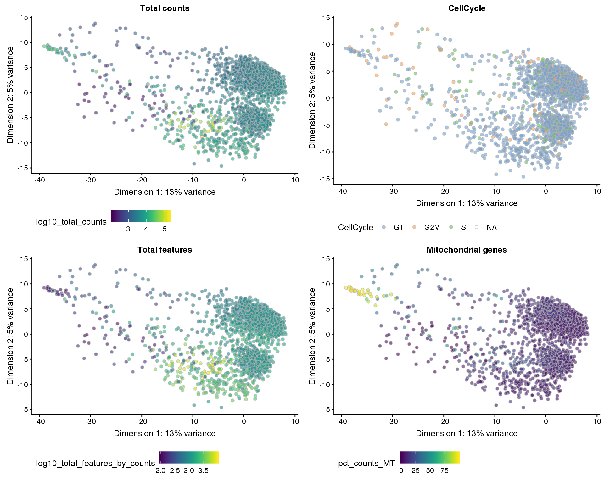

Version	Author	Date
c602800	Luke Zappia	2019-06-20

t-SNE

plot_list <- lapply(names(dimred_factors), function(fct_name) {
    plotTSNE(sce, colour_by = dimred_factors[fct_name]) +
        ggtitle(fct_name) +
        theme(legend.position = "bottom")
})
plot_grid(plotlist = plot_list, ncol = 2)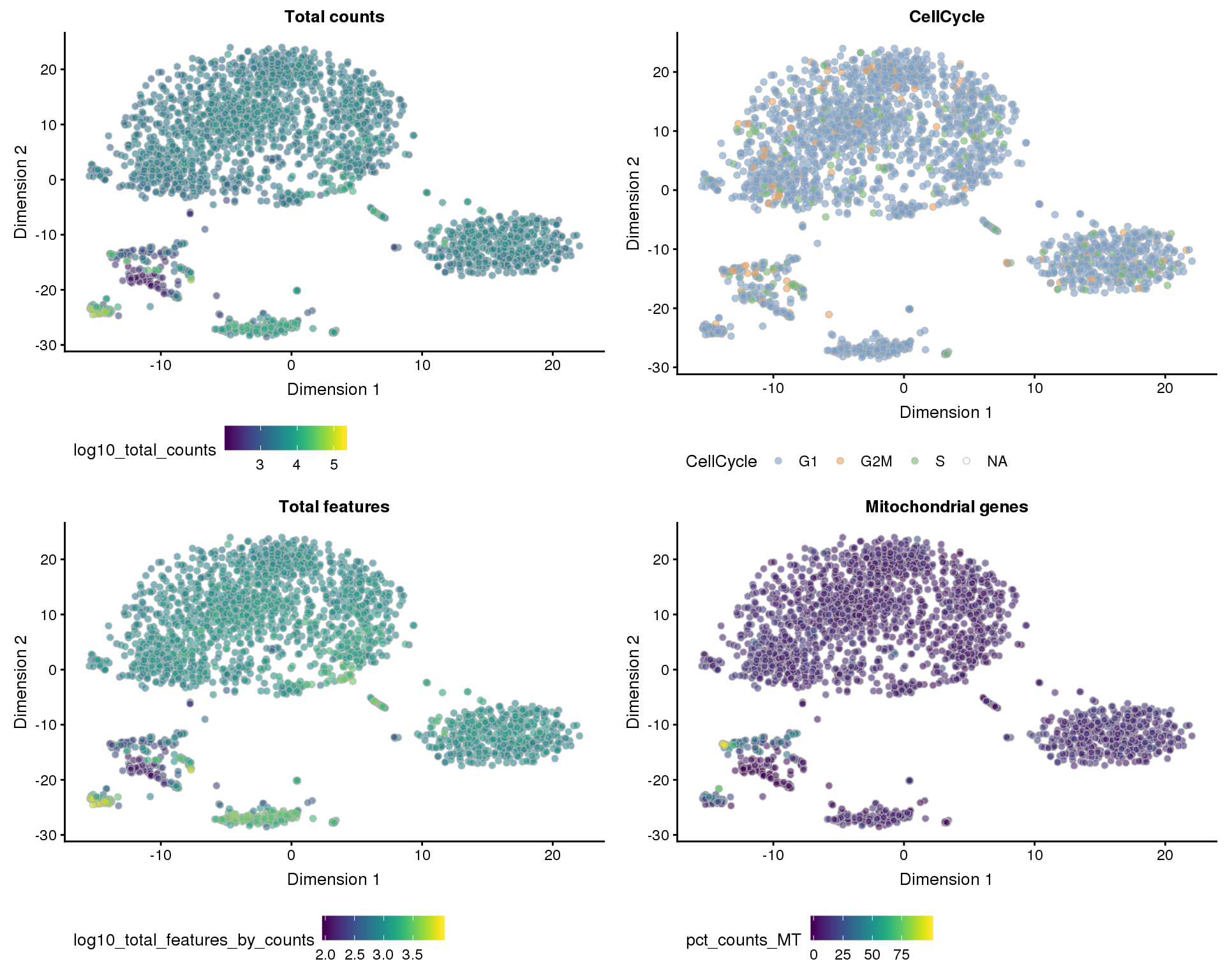

Version	Author	Date
c602800	Luke Zappia	2019-06-20

Explanatory variables

This plot shows the percentage of variance in the dataset that is explained by various technical factors.

exp_vars <- c("CellCycle", "log10_total_counts",
              "pct_counts_in_top_100_features", "total_features_by_counts",
              "pct_counts_MT")
all_zero <- Matrix::rowSums(counts(sce)) == 0
plotExplanatoryVariables(sce[!all_zero, ], variables = exp_vars)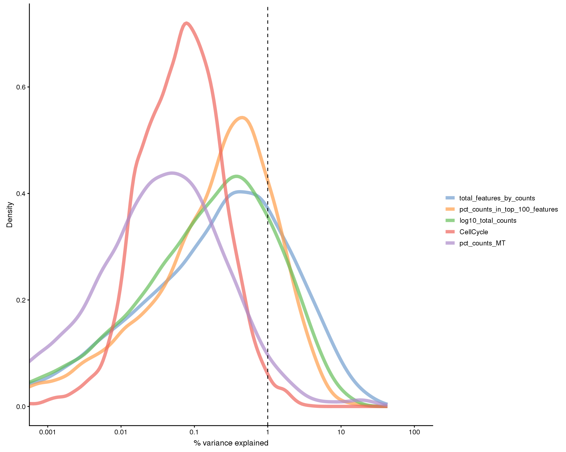

Version	Author	Date
c602800	Luke Zappia	2019-06-20

Cell cycle

The dataset has already been scored for cell cycle activity. This plot shows the G2/M score against the G1 score for each cell and let’s us see the balance of cell cycle phases in the dataset.

ggplot(col_data, aes(x = G1Score, y = G2MScore, colour = CellCycle)) +
    geom_point() +
    xlab("G1 score") +
    ylab("G2/M score") +
    theme_minimal()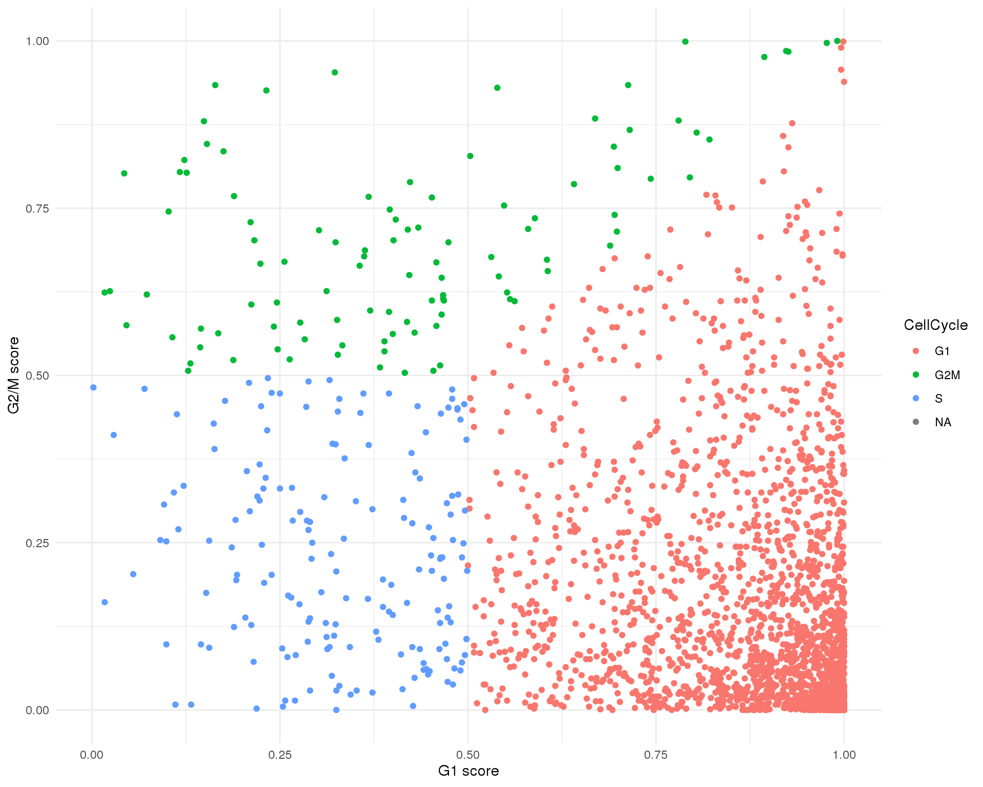

Version	Author	Date
c602800	Luke Zappia	2019-06-20

kable(table(Phase = col_data$CellCycle, useNA = "ifany"))

Phase	Freq
G1	2120
G2M	104
S	174
NA	1

Expression by gene

Distributions by cell. Blue line shows the median and red lines show median absolute deviations (MADs) from the median. We show distributions for all genes and those that have at least one count.

Mean

outlier_histogram(row_data, "log10_mean_counts", mads = c(10, 20))

Version	Author	Date
c602800	Luke Zappia	2019-06-20

Total

outlier_histogram(row_data, "log10_total_counts", mads = 1:5)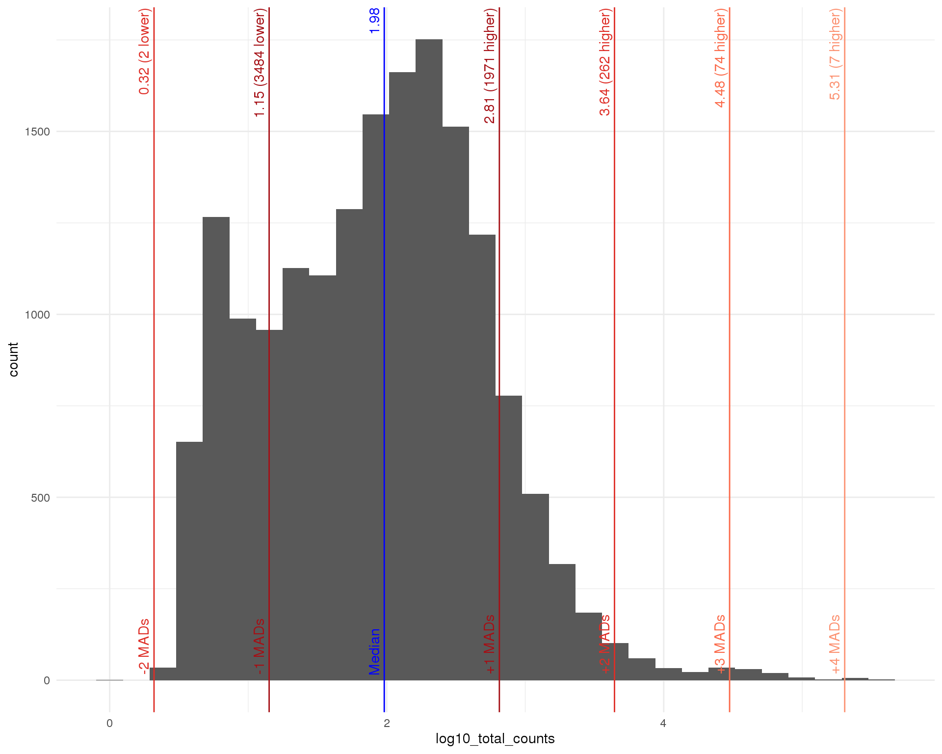

Version	Author	Date
c602800	Luke Zappia	2019-06-20

Mean (expressed)

outlier_histogram(row_data[row_data$total_counts > 0, ],
                  "log10_mean_counts", mads = c(10, 20))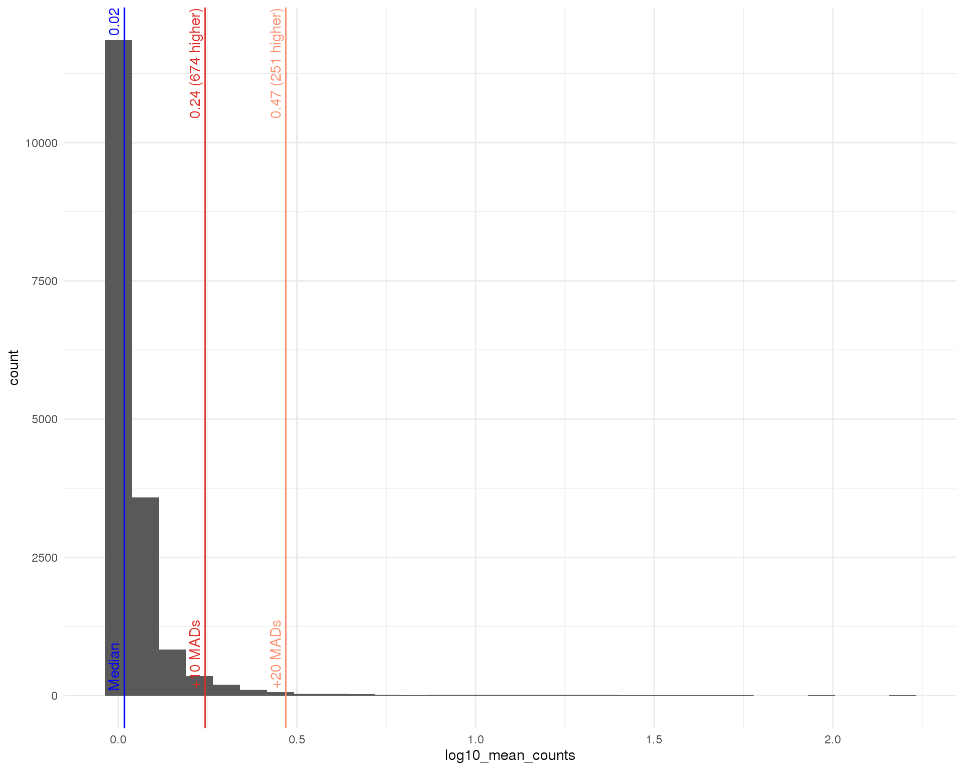

Version	Author	Date
c602800	Luke Zappia	2019-06-20

Total (expressed)

outlier_histogram(row_data[row_data$total_counts > 0, ],
                  "log10_total_counts", mads = 1:5)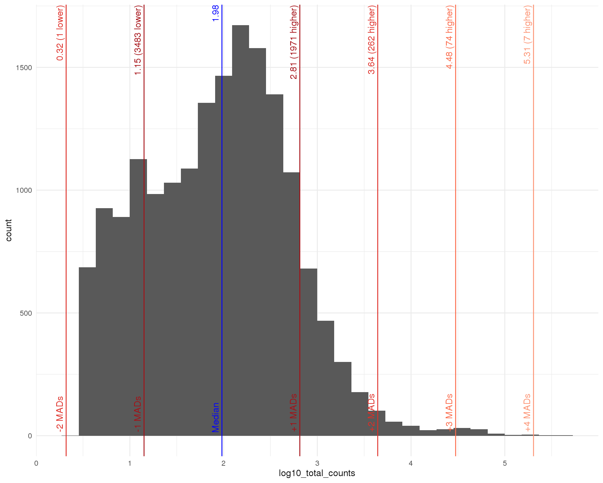

Version	Author	Date
c602800	Luke Zappia	2019-06-20

High expression genes

We can also look at the expression levels of just the top 50 most expressed genes.

plotHighestExprs(sce)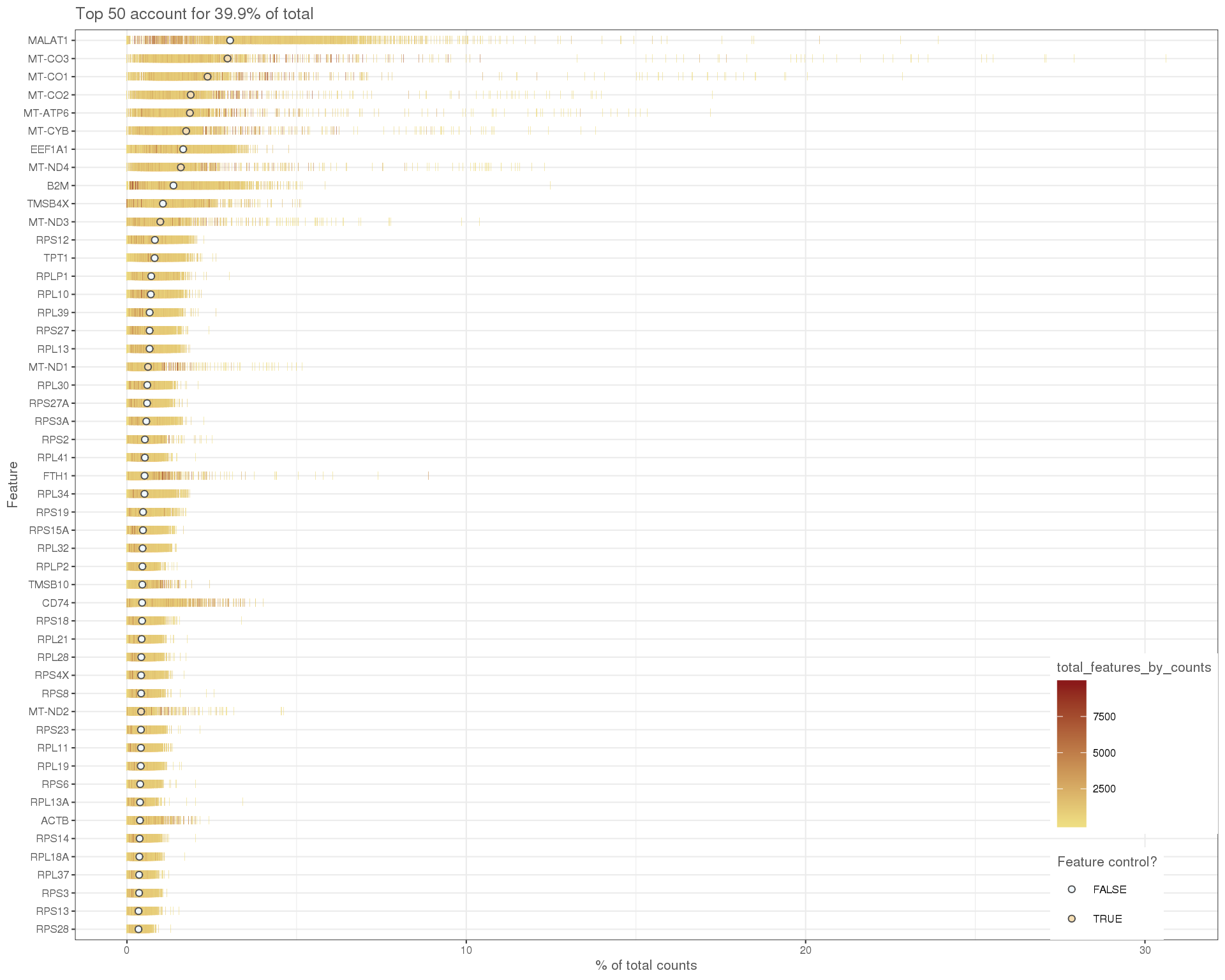

Version	Author	Date
c602800	Luke Zappia	2019-06-20

Expression frequency

The relationshop between the number of cells that express a gene and the overall expression level can also be interesting. We expect to see that higher expressed genes are expressed in more cells but there will also be some that stand out from this.

Frequency by mean

plotExprsFreqVsMean(sce, controls = NULL)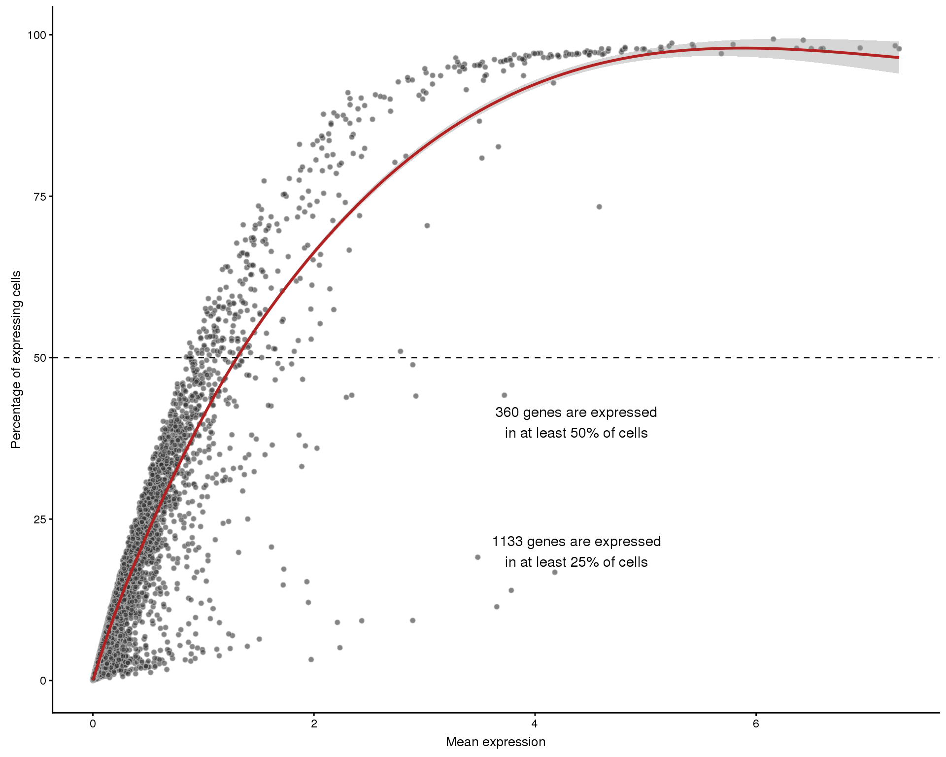

Version	Author	Date
c602800	Luke Zappia	2019-06-20

Zeros by total counts

ggplot(row_data,
       aes(x = log10_total_counts, y = 1 - n_cells_by_counts / nrow(sce),
           colour = gene_biotype)) +
    geom_point(alpha = 0.2, size = 1) +
    scale_y_continuous(labels = scales::percent) +
    ggtitle("Percentage zeros by expression") +
    xlab("log(total counts)") +
    ylab("Percentage zeros")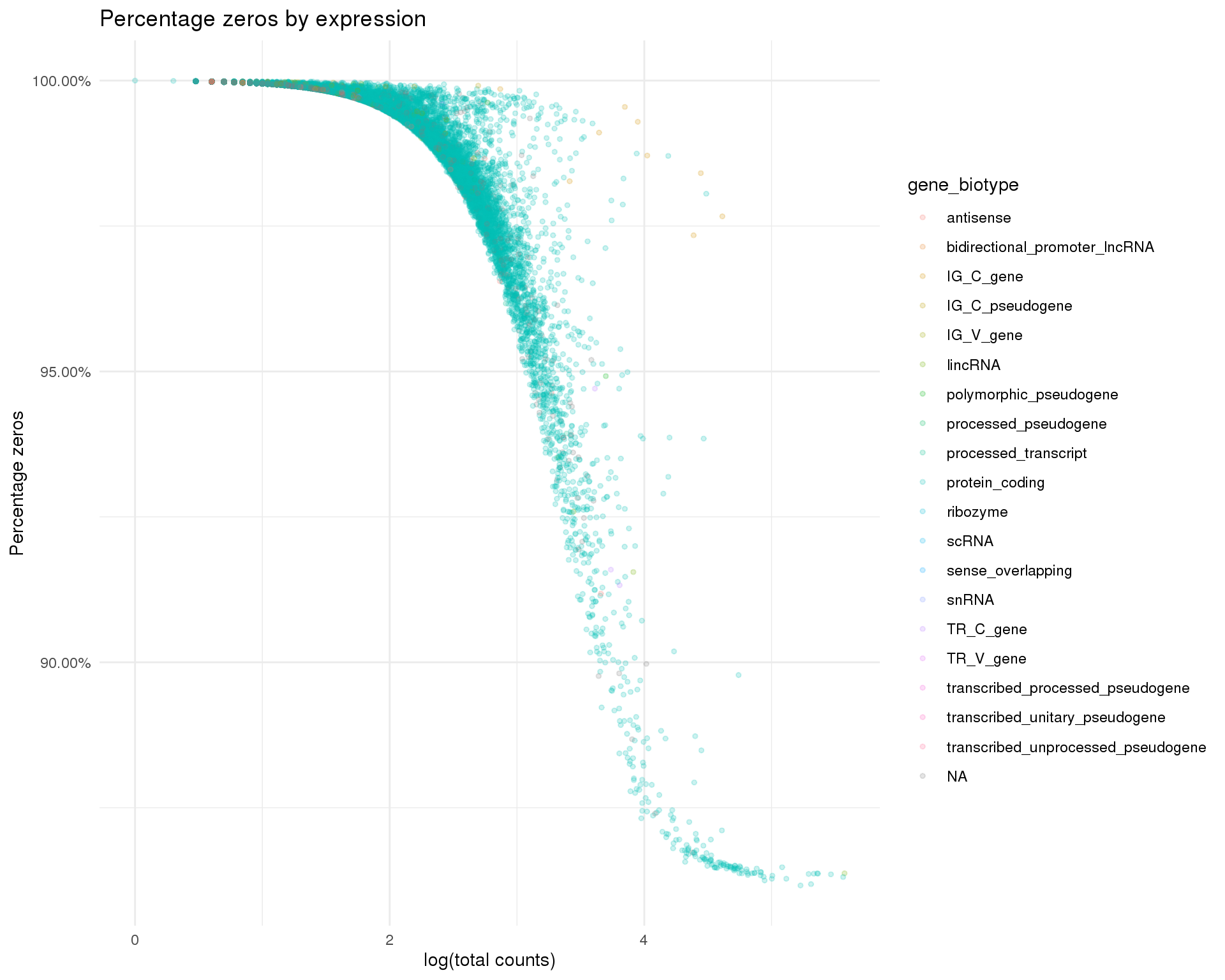

Version	Author	Date
c602800	Luke Zappia	2019-06-20

Cell filtering

We will now perform filtering to select high quality cells. Before we start we have 2399 cells.

The simplest filtering method is to set thresholds on some of the factors we have explored. Specifically these are the total number of counts per cell, the number of features expressed in each cell and the percentage of counts assigned to genes on the mitochondrial chromosome which is used as a proxy for cell damage. The selected thresholds and numbers of filtered cells using this method are:

counts_mads   <- 4
features_mads <- 4
mt_mads       <- 3

counts_out   <- isOutlier(col_data$log10_total_counts,
                          nmads = counts_mads, type = "lower")
features_out <- isOutlier(col_data$log10_total_features_by_counts,
                          nmads = features_mads, type = "lower")
mt_out       <- isOutlier(col_data$pct_counts_MT,
                          nmads = mt_mads, type = "higher")
cite_zero    <- colSums(counts(cite)) == 0

counts_thresh   <- attr(counts_out, "thresholds")["lower"]
features_thresh <- attr(features_out, "thresholds")["lower"]
mt_thresh       <- attr(mt_out, "thresholds")["higher"]

kept <- !(counts_out | features_out | mt_out | cite_zero)
col_data$Kept <- kept

kable(tibble(
    Type = c(
        "Total counts",
        "Total features",
        "Mitochondrial %",
        "CITE counts",
        "Kept cells"
    ),
    Threshold = c(
        paste("< 10 ^", round(counts_thresh, 2),
              paste0("(", round(10 ^ counts_thresh), ")")),
        paste("< 10 ^", round(features_thresh, 2),
              paste0("(", round(10 ^ features_thresh), ")")),
        paste(">", round(mt_thresh, 2), "%"),
        "> 0",
        ""
    ),
    Count = c(
        sum(counts_out),
        sum(features_out),
        sum(mt_out),
        sum(cite_zero),
        sum(kept)
    )
))

Type	Threshold	Count
Total counts	< 10 ^ 2.91 (811)	78
Total features	< 10 ^ 2.61 (411)	112
Mitochondrial %	> 18.77 %	154
CITE counts	> 0	17
Kept cells		2171

colData(sce) <- DataFrame(col_data)
sce_qc <- sce[, kept]
col_data <- col_data[kept, ]

We also remove cells that have no counts in the CITE data. Our filtered dataset now has 2171 cells.

Gene filtering

We also want to perform som filtering of features to remove lowly expressed genes that increase the computation required and may not meet the assumptions of some methods. Let’s look as some distributions now that we have removed low-quality cells.

Distributions

Average counts

avg_counts <- calcAverage(sce_qc, use_size_factors = FALSE)
row_data$AvgCount <- avg_counts
row_data$Log10AvgCount <- log10(avg_counts)
outlier_histogram(row_data, "Log10AvgCount", mads = 1:3, bins = 100)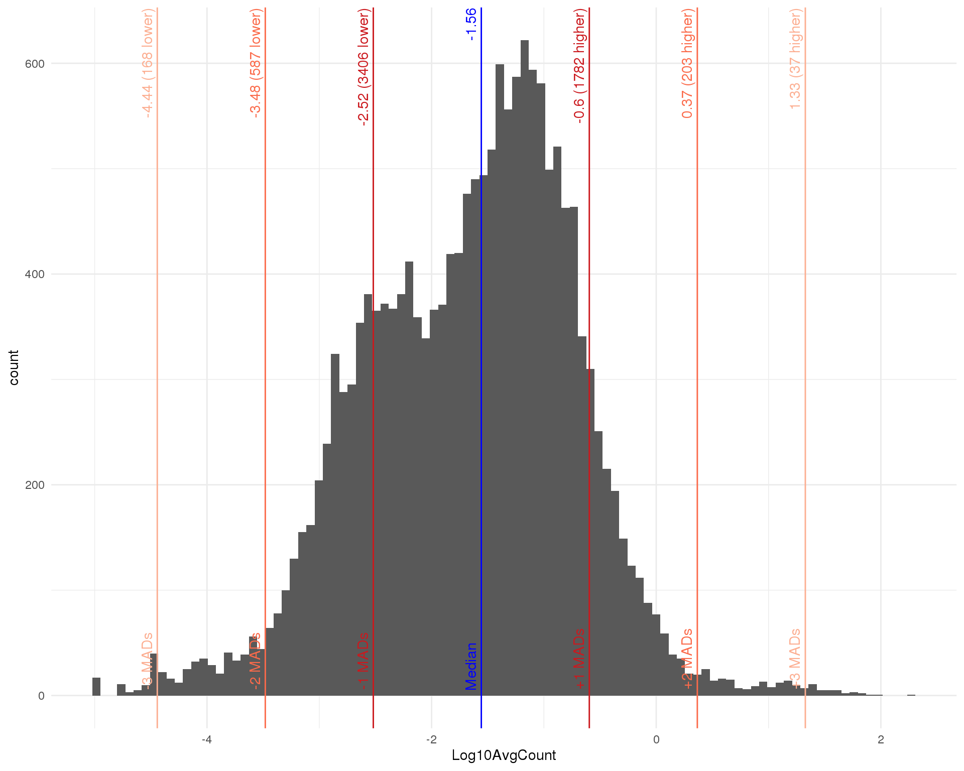

Version	Author	Date
c602800	Luke Zappia	2019-06-20

Number of cells

outlier_histogram(row_data, "n_cells_by_counts", mads = 1:3, bins = 100) +
    scale_x_log10()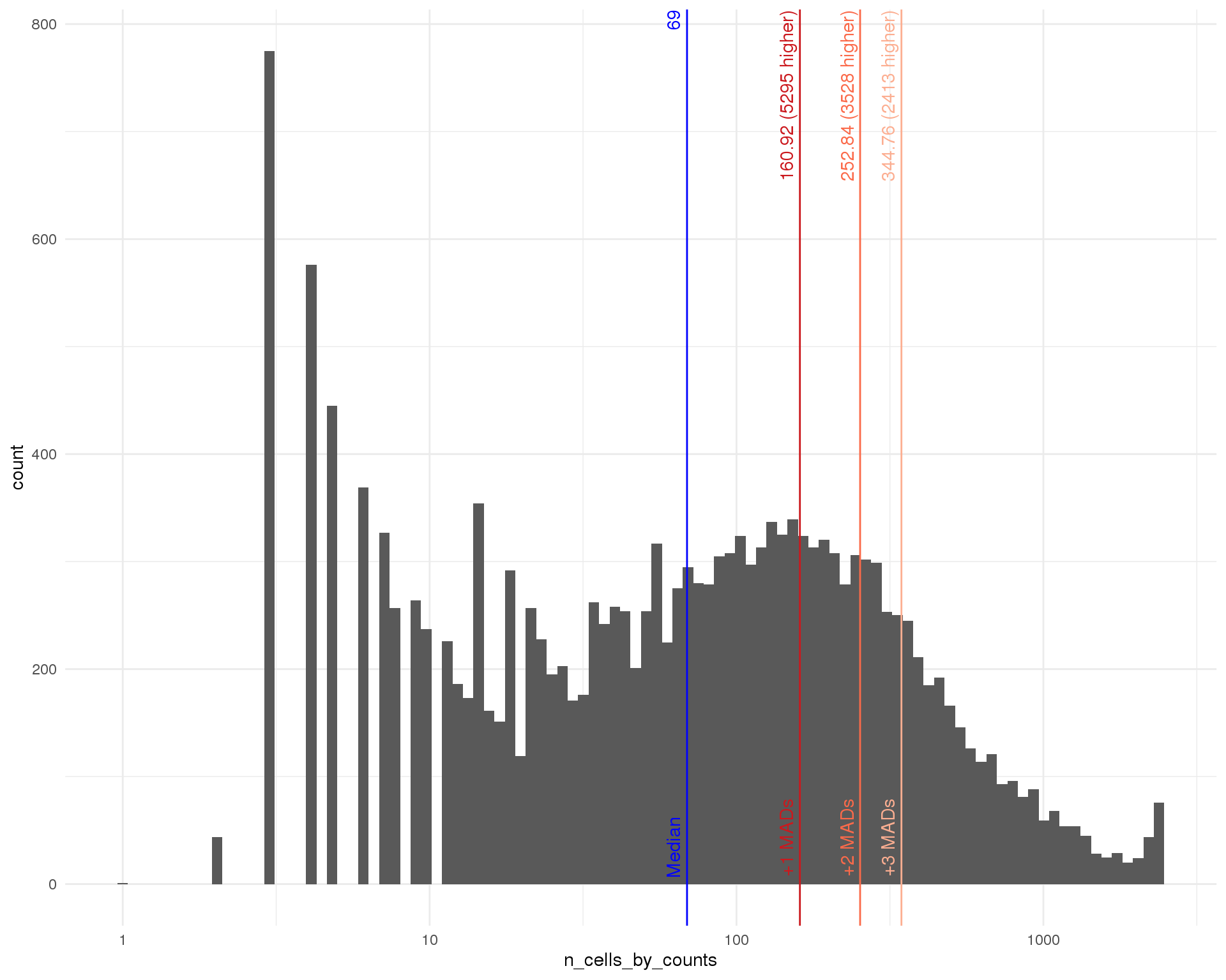

Version	Author	Date
c602800	Luke Zappia	2019-06-20

Filter

min_count <- 1
min_cells <- 2
keep <- Matrix::rowSums(counts(sce_qc) >= min_count) >= min_cells

rowData(sce_qc) <- DataFrame(row_data)
sce_qc <- sce_qc[keep, ]
row_data <- row_data[keep, ]

set.seed(1)
sizeFactors(sce_qc) <- librarySizeFactors(sce_qc)
sce_qc <- normalize(sce_qc)
sce_qc <- runPCA(sce_qc)
sce_qc <- runTSNE(sce_qc)
#sce_qc <- runUMAP(sce_qc)

We use a minimal filter that keeps genes with at least 1 counts in at least 2 cells. After filtering we have reduced the number of features from 17222 to 16859.

Validation

The final quality control step is to inspect some validation plots that should help us see if we need to make any adjustments.

Kept vs lost

One thing we can look at is the difference in expression between the kept and removed cells. If we see known genes that are highly expressed in the removed cells that can indicate that we have removed an interesting population of cells from the dataset. The red line shows equal expression and the blue line is a linear fit.

pass_qc <- colnames(sce) %in% colnames(sce_qc)
lost_counts <- counts(sce)[, !pass_qc]
kept_counts <- counts(sce)[,  pass_qc]

kept_lost <- tibble(
    Gene     = rownames(sce),
    Lost     = calcAverage(lost_counts),
    LostProp = Matrix::rowSums(lost_counts > 0) / ncol(lost_counts),
    Kept     = calcAverage(kept_counts),
    KeptProp = Matrix::rowSums(kept_counts > 0) / ncol(kept_counts)
) %>%
    mutate(LogFC = predFC(cbind(Lost, Kept),
                          design = cbind(1, c(1, 0)))[, 2]) %>%
    mutate(LostCapped = pmax(Lost, min(Lost[Lost > 0]) * 0.5),
           KeptCapped = pmax(Kept, min(Kept[Kept > 0]) * 0.5))

ggplot(kept_lost,
       aes(x = LostCapped, y = KeptCapped, colour = LostProp - KeptProp)) +
    geom_point(size = 1, alpha = 0.2) +
    geom_abline(intercept = 0, slope = 1, colour = "red") +
    geom_smooth(method = "lm") +
    scale_x_log10() +
    scale_y_log10() +
    scale_colour_viridis_c() +
    ggtitle("Gene expression in kept and removed cells") +
    xlab("Average count (removed)") +
    ylab("Average count (kept)") +
    theme_minimal()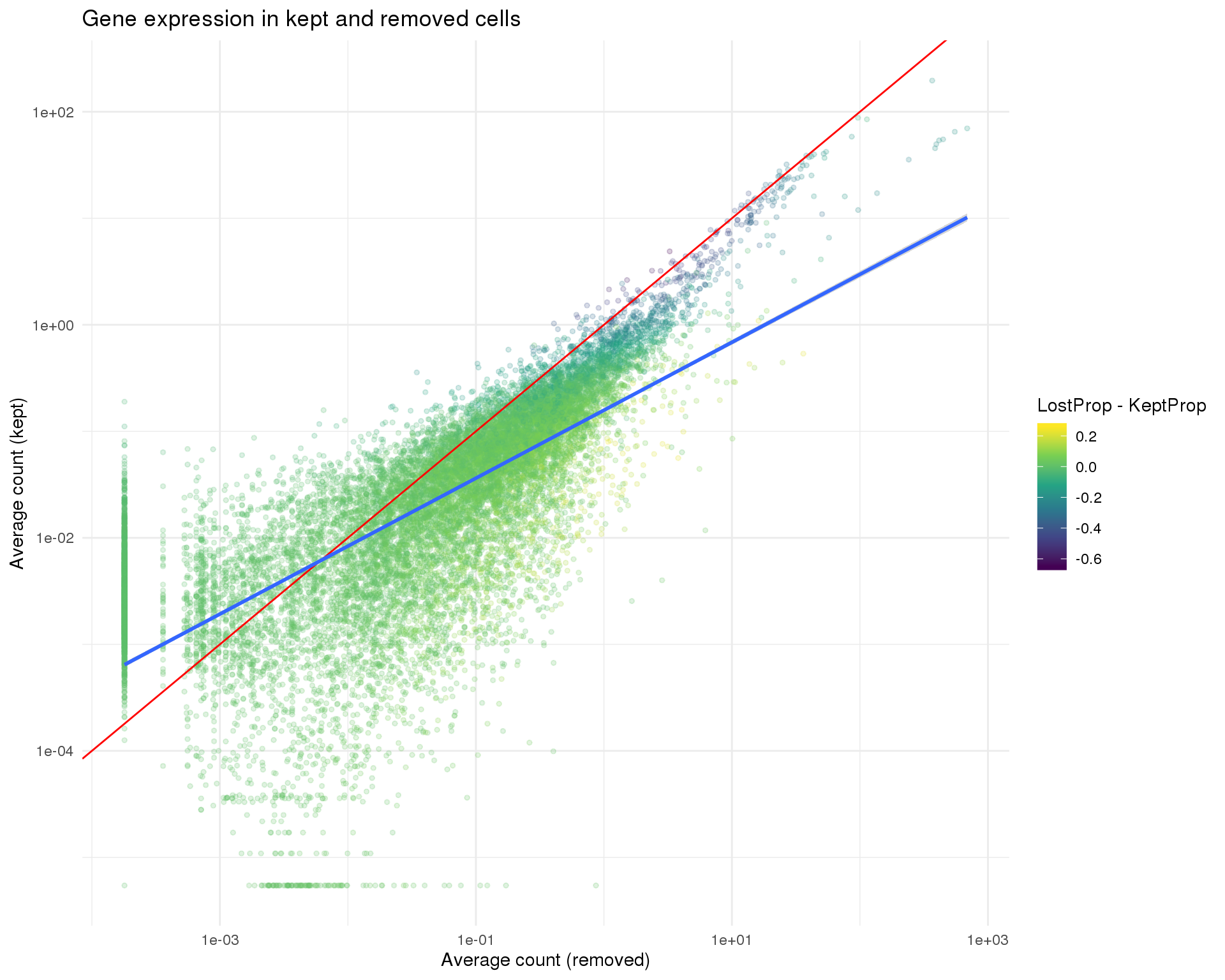

Version	Author	Date
c602800	Luke Zappia	2019-06-20

kept_lost %>%
    select(Gene, LogFC, Lost, LostProp, Kept, KeptProp) %>%
    arrange(-LogFC) %>%
    as.data.frame() %>%
    head(100)

Dimensionality reduction

Dimsionality reduction plots coloured by technical factors again gives us a good overview of the dataset.

PCA

plot_list <- lapply(names(dimred_factors), function(fct_name) {
    plotPCA(sce_qc, colour_by = dimred_factors[fct_name]) +
        ggtitle(fct_name) +
        theme(legend.position = "bottom")
})
plot_grid(plotlist = plot_list, ncol = 2)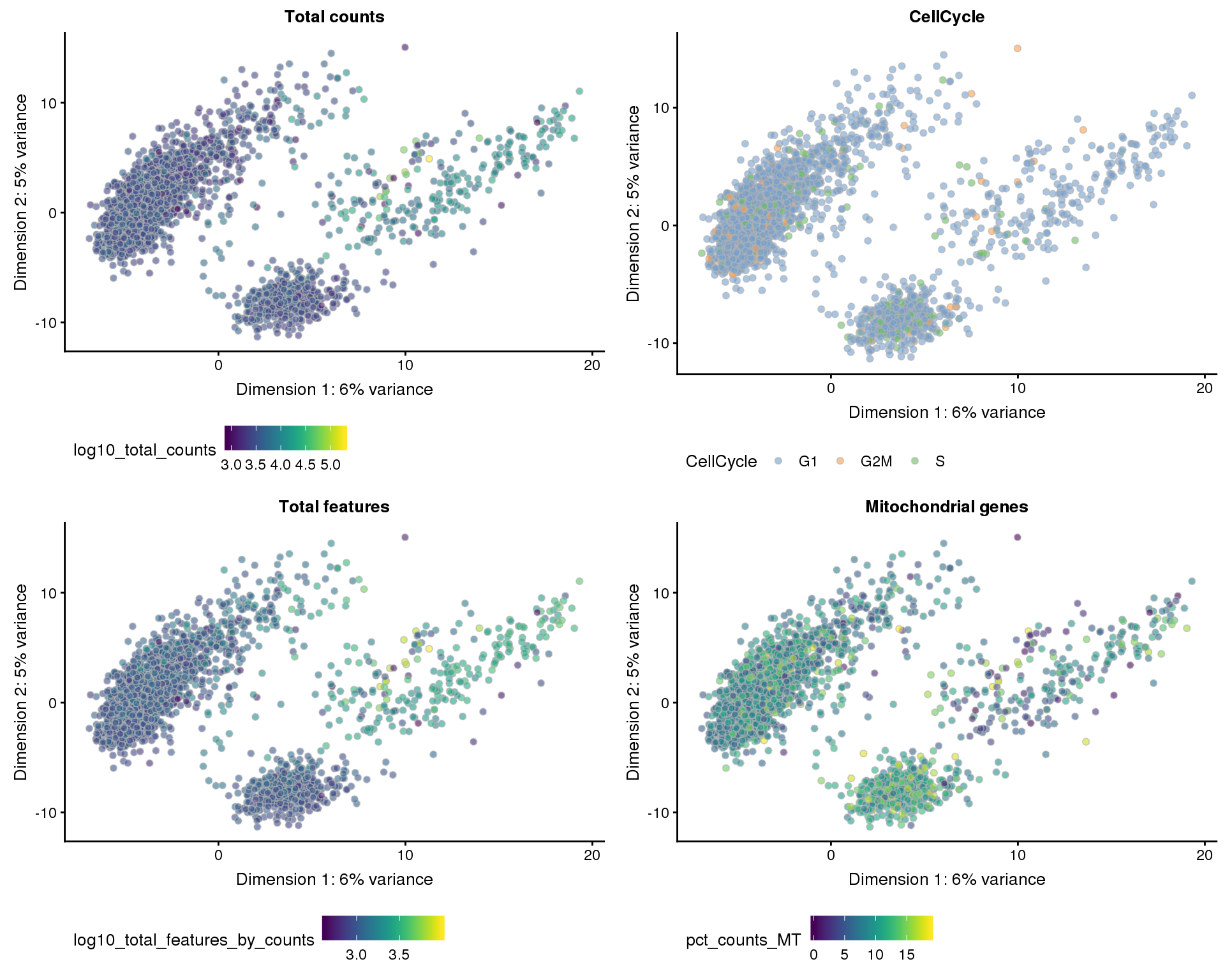

Version	Author	Date
c602800	Luke Zappia	2019-06-20

t-SNE

plot_list <- lapply(names(dimred_factors), function(fct_name) {
    plotTSNE(sce_qc, colour_by = dimred_factors[fct_name]) +
        ggtitle(fct_name) +
        theme(legend.position = "bottom")
})
plot_grid(plotlist = plot_list, ncol = 2)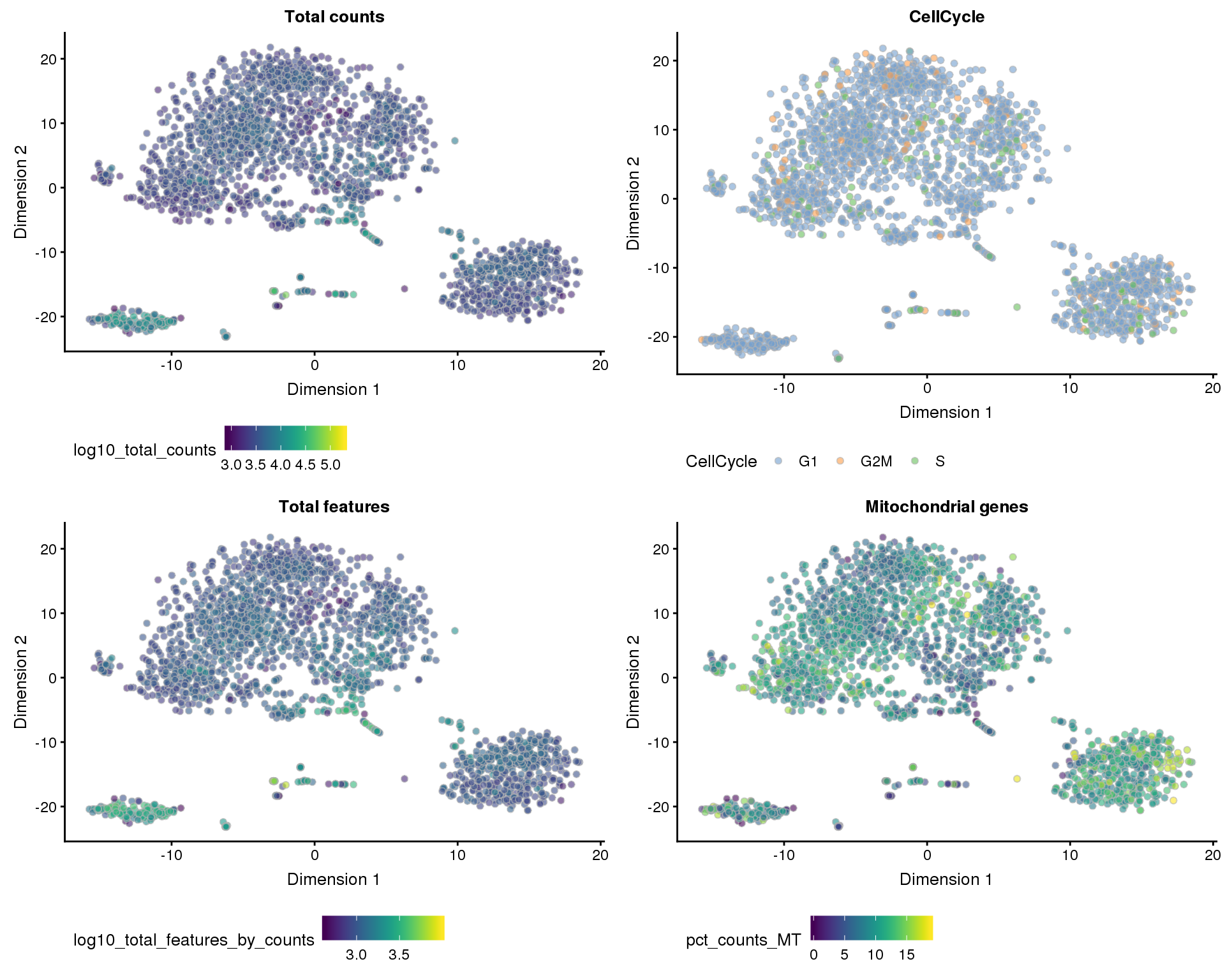

Version	Author	Date
c602800	Luke Zappia	2019-06-20

Filter CITE

We want to select the same set of cells in the CITE data.

cite_qc <- cite[, colnames(sce_qc)]

Summary

After quality control we have a dataset with 2171 cells and 16859 genes.

Parameters

This table describes parameters used and set in this document.

params <- list(
    list(
        Parameter = "counts_thresh",
        Value = counts_thresh,
        Description = "Minimum threshold for (log10) total counts"
    ),
    list(
        Parameter = "features_thresh",
        Value = features_thresh,
        Description = "Minimum threshold for (log10) total features"
    ),
    list(
        Parameter = "mt_thresh",
        Value = mt_thresh,
        Description = "Maximum threshold for percentage counts mitochondrial"
    ),
    list(
        Parameter = "counts_mads",
        Value = counts_mads,
        Description = "MADs for (log10) total counts threshold"
    ),
    list(
        Parameter = "features_mads",
        Value = features_mads,
        Description = "MADs for (log10) total features threshold"
    ),
    list(
        Parameter = "mt_mads",
        Value = mt_mads,
        Description = "MADs for percentage counts mitochondrial threshold"
    ),
    list(
        Parameter = "min_count",
        Value = min_count,
        Description = "Minimum count per cell for gene filtering"
    ),
    list(
        Parameter = "min_cells",
        Value = min_cells,
        Description = "Minimum cells with min_count counts for gene filtering"
    ),
    list(
        Parameter = "n_cells",
        Value = ncol(sce_qc),
        Description = "Number of cells in the filtered dataset"
    ),
    list(
        Parameter = "n_genes",
        Value = nrow(sce_qc),
        Description = "Number of genes in the filtered dataset"
    ),
    list(
        Parameter = "median_genes",
        Value = median(Matrix::colSums(counts(sce_qc) != 0)),
        Description = paste("Median number of expressed genes per cell in the",
                            "filtered dataset")
    ),
    list(
        Parameter = "median_counts",
        Value = median(Matrix::colSums(counts(sce_qc))),
        Description = paste("Median number of counts per cell in the filtered",
                            "dataset")
    )
)
params <- toJSON(params, pretty = TRUE)
kable(fromJSON(params))

Parameter	Value	Description
counts_thresh	2.909	Minimum threshold for (log10) total counts
features_thresh	2.6136	Minimum threshold for (log10) total features
mt_thresh	18.7663	Maximum threshold for percentage counts mitochondrial
counts_mads	4	MADs for (log10) total counts threshold
features_mads	4	MADs for (log10) total features threshold
mt_mads	3	MADs for percentage counts mitochondrial threshold
min_count	1	Minimum count per cell for gene filtering
min_cells	2	Minimum cells with min_count counts for gene filtering
n_cells	2171	Number of cells in the filtered dataset
n_genes	16859	Number of genes in the filtered dataset
median_genes	1066	Median number of expressed genes per cell in the filtered dataset
median_counts	3226	Median number of counts per cell in the filtered dataset

Output files

This table describes the output files produced by this document. Right click and Save Link As… to download the results.

write_rds(sce_qc, PATHS$sce_qc, compress = "bz", compression = 9)
write_rds(cite_qc, PATHS$cite_qc, compress = "bz", compression = 9)
write_lines(params, path(OUT_DIR, "parameters.json"))

kable(data.frame(
    File = c(
        download_link("parameters.json", OUT_DIR)
    ),
    Description = c(
        "Parameters set and used in this analysis"
    )
))

File	Description
parameters.json	Parameters set and used in this analysis

Session information

sessioninfo::session_info()

─ Session info ──────────────────────────────────────────────────────────
 setting  value                       
 version  R version 3.6.0 (2019-04-26)
 os       CentOS release 6.7 (Final)  
 system   x86_64, linux-gnu           
 ui       X11                         
 language (EN)                        
 collate  en_US.UTF-8                 
 ctype    en_US.UTF-8                 
 tz       Australia/Melbourne         
 date     2019-06-26                  

─ Packages ──────────────────────────────────────────────────────────────
 ! package              * version   date       lib source        
   assertthat             0.2.1     2019-03-21 [1] CRAN (R 3.6.0)
   backports              1.1.4     2019-04-10 [1] CRAN (R 3.6.0)
   beeswarm               0.2.3     2016-04-25 [1] CRAN (R 3.6.0)
   Biobase              * 2.44.0    2019-05-02 [1] Bioconductor  
   BiocGenerics         * 0.30.0    2019-05-02 [1] Bioconductor  
   BiocNeighbors          1.2.0     2019-05-02 [1] Bioconductor  
   BiocParallel         * 1.18.0    2019-05-03 [1] Bioconductor  
   BiocSingular           1.0.0     2019-05-02 [1] Bioconductor  
   bitops                 1.0-6     2013-08-17 [1] CRAN (R 3.6.0)
   broom                  0.5.2     2019-04-07 [1] CRAN (R 3.6.0)
   cellranger             1.1.0     2016-07-27 [1] CRAN (R 3.6.0)
   cli                    1.1.0     2019-03-19 [1] CRAN (R 3.6.0)
   colorspace             1.4-1     2019-03-18 [1] CRAN (R 3.6.0)
   conflicted           * 1.0.3     2019-05-01 [1] CRAN (R 3.6.0)
   cowplot              * 0.9.4     2019-01-08 [1] CRAN (R 3.6.0)
   crayon                 1.3.4     2017-09-16 [1] CRAN (R 3.6.0)
   DelayedArray         * 0.10.0    2019-05-02 [1] Bioconductor  
   DelayedMatrixStats     1.6.0     2019-05-02 [1] Bioconductor  
   digest                 0.6.19    2019-05-20 [1] CRAN (R 3.6.0)
   dplyr                * 0.8.1     2019-05-14 [1] CRAN (R 3.6.0)
   edgeR                * 3.26.4    2019-05-27 [1] Bioconductor  
   evaluate               0.14      2019-05-28 [1] CRAN (R 3.6.0)
   forcats              * 0.4.0     2019-02-17 [1] CRAN (R 3.6.0)
   fs                   * 1.3.1     2019-05-06 [1] CRAN (R 3.6.0)
   generics               0.0.2     2018-11-29 [1] CRAN (R 3.6.0)
   GenomeInfoDb         * 1.20.0    2019-05-02 [1] Bioconductor  
   GenomeInfoDbData       1.2.1     2019-06-19 [1] Bioconductor  
   GenomicRanges        * 1.36.0    2019-05-02 [1] Bioconductor  
   ggbeeswarm             0.6.0     2017-08-07 [1] CRAN (R 3.6.0)
   ggplot2              * 3.2.0     2019-06-16 [1] CRAN (R 3.6.0)
   git2r                  0.25.2    2019-03-19 [1] CRAN (R 3.6.0)
   glue                   1.3.1     2019-03-12 [1] CRAN (R 3.6.0)
   gridExtra              2.3       2017-09-09 [1] CRAN (R 3.6.0)
   gtable                 0.3.0     2019-03-25 [1] CRAN (R 3.6.0)
   haven                  2.1.0     2019-02-19 [1] CRAN (R 3.6.0)
   here                 * 0.1       2017-05-28 [1] CRAN (R 3.6.0)
   highr                  0.8       2019-03-20 [1] CRAN (R 3.6.0)
   hms                    0.4.2     2018-03-10 [1] CRAN (R 3.6.0)
   htmltools              0.3.6     2017-04-28 [1] CRAN (R 3.6.0)
   httr                   1.4.0     2018-12-11 [1] CRAN (R 3.6.0)
   IRanges              * 2.18.1    2019-05-31 [1] Bioconductor  
   irlba                  2.3.3     2019-02-05 [1] CRAN (R 3.6.0)
   jsonlite             * 1.6       2018-12-07 [1] CRAN (R 3.6.0)
   knitr                * 1.23      2019-05-18 [1] CRAN (R 3.6.0)
   labeling               0.3       2014-08-23 [1] CRAN (R 3.6.0)
 P lattice                0.20-38   2018-11-04 [5] CRAN (R 3.6.0)
   lazyeval               0.2.2     2019-03-15 [1] CRAN (R 3.6.0)
   limma                * 3.40.2    2019-05-17 [1] Bioconductor  
   locfit                 1.5-9.1   2013-04-20 [1] CRAN (R 3.6.0)
   lubridate              1.7.4     2018-04-11 [1] CRAN (R 3.6.0)
   magrittr               1.5       2014-11-22 [1] CRAN (R 3.6.0)
 P Matrix                 1.2-17    2019-03-22 [5] CRAN (R 3.6.0)
   matrixStats          * 0.54.0    2018-07-23 [1] CRAN (R 3.6.0)
   memoise                1.1.0     2017-04-21 [1] CRAN (R 3.6.0)
 P mgcv                   1.8-28    2019-03-21 [5] CRAN (R 3.6.0)
   modelr                 0.1.4     2019-02-18 [1] CRAN (R 3.6.0)
   munsell                0.5.0     2018-06-12 [1] CRAN (R 3.6.0)
 P nlme                   3.1-139   2019-04-09 [5] CRAN (R 3.6.0)
   pillar                 1.4.1     2019-05-28 [1] CRAN (R 3.6.0)
   pkgconfig              2.0.2     2018-08-16 [1] CRAN (R 3.6.0)
   purrr                * 0.3.2     2019-03-15 [1] CRAN (R 3.6.0)
   R6                     2.4.0     2019-02-14 [1] CRAN (R 3.6.0)
   RColorBrewer           1.1-2     2014-12-07 [1] CRAN (R 3.6.0)
   Rcpp                   1.0.1     2019-03-17 [1] CRAN (R 3.6.0)
   RCurl                  1.95-4.12 2019-03-04 [1] CRAN (R 3.6.0)
   readr                * 1.3.1     2018-12-21 [1] CRAN (R 3.6.0)
   readxl                 1.3.1     2019-03-13 [1] CRAN (R 3.6.0)
   rlang                  0.3.4     2019-04-07 [1] CRAN (R 3.6.0)
   rmarkdown              1.13      2019-05-22 [1] CRAN (R 3.6.0)
   rprojroot              1.3-2     2018-01-03 [1] CRAN (R 3.6.0)
   rstudioapi             0.10      2019-03-19 [1] CRAN (R 3.6.0)
   rsvd                   1.0.1     2019-06-02 [1] CRAN (R 3.6.0)
   Rtsne                  0.15      2018-11-10 [1] CRAN (R 3.6.0)
   rvest                  0.3.4     2019-05-15 [1] CRAN (R 3.6.0)
   S4Vectors            * 0.22.0    2019-05-02 [1] Bioconductor  
   scales                 1.0.0     2018-08-09 [1] CRAN (R 3.6.0)
   scater               * 1.12.2    2019-05-24 [1] Bioconductor  
   sessioninfo            1.1.1     2018-11-05 [1] CRAN (R 3.6.0)
   SingleCellExperiment * 1.6.0     2019-05-02 [1] Bioconductor  
   stringi                1.4.3     2019-03-12 [1] CRAN (R 3.6.0)
   stringr              * 1.4.0     2019-02-10 [1] CRAN (R 3.6.0)
   SummarizedExperiment * 1.14.0    2019-05-02 [1] Bioconductor  
   tibble               * 2.1.3     2019-06-06 [1] CRAN (R 3.6.0)
   tidyr                * 0.8.3     2019-03-01 [1] CRAN (R 3.6.0)
   tidyselect             0.2.5     2018-10-11 [1] CRAN (R 3.6.0)
   tidyverse            * 1.2.1     2017-11-14 [1] CRAN (R 3.6.0)
   vipor                  0.4.5     2017-03-22 [1] CRAN (R 3.6.0)
   viridis                0.5.1     2018-03-29 [1] CRAN (R 3.6.0)
   viridisLite            0.3.0     2018-02-01 [1] CRAN (R 3.6.0)
   whisker                0.3-2     2013-04-28 [1] CRAN (R 3.6.0)
   withr                  2.1.2     2018-03-15 [1] CRAN (R 3.6.0)
   workflowr              1.4.0     2019-06-08 [1] CRAN (R 3.6.0)
   xfun                   0.7       2019-05-14 [1] CRAN (R 3.6.0)
   xml2                   1.2.0     2018-01-24 [1] CRAN (R 3.6.0)
   XVector                0.24.0    2019-05-02 [1] Bioconductor  
   yaml                   2.2.0     2018-07-25 [1] CRAN (R 3.6.0)
   zlibbioc               1.30.0    2019-05-02 [1] Bioconductor  

[1] /group/bioi1/luke/analysis/OzSingleCells2019/packrat/lib/x86_64-pc-linux-gnu/3.6.0
[2] /group/bioi1/luke/analysis/OzSingleCells2019/packrat/lib-ext/x86_64-pc-linux-gnu/3.6.0
[3] /group/bioi1/luke/analysis/OzSingleCells2019/packrat/lib-R/x86_64-pc-linux-gnu/3.6.0
[4] /home/luke.zappia/R/x86_64-pc-linux-gnu-library/3.6
[5] /usr/local/installed/R/3.6.0/lib64/R/library

 P ── Loaded and on-disk path mismatch.

Quality control

2019-06-26

Introduction

Exploration

Expression by cell

Total counts

Total features

Percent mitochondrial

Dimensionality reduction

PCA

t-SNE

Explanatory variables

Cell cycle

Expression by gene

Mean

Total

Mean (expressed)

Total (expressed)

High expression genes

Expression frequency

Frequency by mean

Zeros by total counts

Cell filtering

Gene filtering

Distributions

Average counts

Number of cells

Filter

Validation

Kept vs lost

Dimensionality reduction

PCA

t-SNE

Filter CITE

Summary

Parameters

Output files

Session information